This section presents the design of the questionnaire used in the survey pilot, which may differ from the questionnaire to be used in the first wave. Considering that, this chapter is divided into four sections:
First, the ethical considerations for the proper administration of the survey are presented, clarifying the information related to informed consent and the institutional approvals required for administering the instrument. Next, the sections of the survey are presented, detailing separately the assignment task, the attitudinal items, and the socioeconomic characterization questions, providing a more in-depth look at the item scales that were used, their origin, and measurement specifications.
3.1 Ethics certification and informed consent
The research project, as well as the survey, was submitted for review to the Research Ethics Committee of the Faculty of Social Sciences at the University of Chile and was approved under number 23-33/2025.
To conduct the survey, an informed consent form was developed that details the questionnaire administration process; this form must be provided to respondents to obtain their consent to participate in the survey.
3.2 Distributive Conjoint-Survey experiment
This section describes the core element of the survey: the design and implementation of the distributive conjoint module. This module is based on a distributive design, which is a type of survey experiment that allows researchers to study how people allocate scarce resources among competing claimants. In this case, the scarce resource is a fixed scholarship fund, and the competing claimants are two applicants with different attributes. The design allows researchers to examine how respondents make trade-offs between different attributes of the applicants, such as their academic performance, financial need, and personal characteristics. In this case, the attributes of the applicants are operationalized based on the CARIN and recast NICER frameworks, which are widely used in the welfare deservingness literature. The design also allows researchers to test hypotheses about how different attributes of the applicants affect respondents’ allocation decisions, and how these decisions are influenced by respondents’ own characteristics and beliefs.
The design adapts the Distributional Survey Experiment of Gilgen (2022) to a conjoint format (Hainmueller et al., 2014), combining the tabular presentation and complete, independent randomization of a conjoint experiment with the fixed-sum allocation task characteristic of distributive designs. The applicant attributes operationalize deservingness criteria drawn from the welfare deservingness literature, specifically the CARIN and recast NICER frameworks (Knotz et al., 2022; Meuleman et al., 2020; Oorschot, 2000); the theoretical rationale for each attribute, the derivation of the hypotheses, and the analysis plan are documented separately in the Pre Analysis Plan.
This section is organized in the following subsections:
Task design and randomization
Analysis considerations
Power analysis
3.2.1 Task design and randomization
The study uses a paired-profile distributive conjoint, a design that fuses the randomization logic of conjoint survey experiments with the allocative logic of distributive justice experiments. As in a standard conjoint, each task presents two profiles whose attributes are independently randomized, and the analysis recovers the effect of each attribute and level on the outcome. What departs from the standard conjoint is the response: rather than choosing one profile over the other, the respondent distributes a fixed resource between them, allocating a percentage of the total to each. The design therefore functions as an allocator—it asks how a scarce good should be divided between two independent claimants—and reveals the weight respondents place on each attribute through the share they are willing to grant.
Attributes and levels {#sec-attributes}
The profiles are defined by seven attributes, which operationalize six deservingness criteria (need, identity, control, effort, reciprocity, and attitude), and one additional attribute (sex of the applicant). Two of the deservingness criteria are operationalized with three levels, while the remaining four are operationalized with two levels.
Attribute
Criterion
Profile label
Levels
Need
Need (CARIN/NICER)
Makes ends meet with (Su hogar llega a fin de mes con:)
1 Comfort (Holgura)
2 Hardship (Dificultad)
Identity
Identity (CARIN/NICER)
Country of birth (País de nacimiento:)
1 Chile
2 Peru (Perú)
3 Venezuela
Control
Control (CARIN/NICER)
Needs the scholarship because (Requiere la beca porque:)
1 Did not apply to other scholarships in time (No alcanzó a postular a tiempo a otras becas)
2 Applied to other scholarships but received no funding (Postuló a otras becas pero no obtuvo financiamiento)
Effort
Effort (NICER)
Studies (Estudia:)
1 Less than their peers (Menos que sus compañeros)
2 The same as their peers (Igual que sus compañeros)
3 More than their peers (Más que sus compañeros)
Reciprocity
Reciprocity (CARIN/NICER)
Outside their studies (Fuera de sus estudios:)
1 Has not done volunteer work (No ha hecho voluntariado)
2 Has done volunteer work (Ha hecho voluntariado)
Attitude
Attitude (CARIN)
Sees the scholarship as (Ve la beca como:)
1 Something they deserve (Algo que se merece)
2 Help they are grateful for (Una ayuda que agradece)
Sex
Ascriptive (signaled by name)
First name (no explicit row)
1 Male name
2 Female name
The resulting profiles are presented in a tabular format, with each attribute and its corresponding level displayed in a separate row. The table is designed to be visually clear and easy to read, allowing respondents to quickly compare the two profiles and make their allocation decisions. Besides, the allocation task is performed with a slider that allows respondents to allocate a percentage of the total scholarship fund to each profile, with the constraint that the total allocation must equal 100%. The slider is designed to be intuitive and user-friendly, allowing respondents to easily adjust their allocations and see the resulting changes in real-time.
Considering the number of attributes and levels, the total number of possible profiles is (2x3x2x3x2x2x2) = 288. The total number of possible (non redundant) profile pairs is p(p-1)/2 = (288287)/2 = 41,328. The survey design randomly selects a subset of these pairs to present to respondents, ensuring that each respondent sees a unique combination of profiles.
The experiment uses complete and independent randomization of attribute levels, the reference case in Hainmueller et al. (2014) and the default for most applied conjoint designs (Bansak et al., 2021). For each profile \((j)\), every attribute is drawn independently of the others and of the competing profile, with uniform probability within its attribute (\(1/2\) for the four two-level attributes, \(1/3\) for Effort and Identity). No attribute is conditioned on another and no level is reweighted, so the joint distribution of profiles is the product of the attribute marginals (Hainmueller et al., 2014). Randomization occurs at the profile level and is performed anew for each respondent and task, rather than as a fixed block assigned in advance. Under this scheme the assignment of each attribute is by construction independent of the potential outcomes, which is the condition that identifies the AMCEs (Hainmueller et al., 2014). The randomization is implemented in the survey platform using a custom script that generates the profiles and their corresponding levels on the fly, ensuring that each respondent sees a unique set of profiles.
A direct consequence of independent randomization is orthogonality: across the sample, the level of any one attribute is statistically independent of the level of every other, so the estimated effect of one attribute cannot be biased by the distribution of another. Exact zero correlation holds only in expectation, so it is worth stating what “independent” means at a finite sample. With 54,000 profiles the sampling standard error of a correlation between any two attribute indicators is approximately \(1/\sqrt{54{,}000} \approx 0.004\), so inter-attribute correlations should fall within roughly \(\pm 0.013\) of zero (three standard errors) purely by sampling variation. A simulation of the design under the realized sample size confirms this directly: across the full attribute set the largest observed within-profile correlation is \(0.011\), within the expected band and stable across repeated seeds (see ?sec-random-check). Departures of this magnitude are sampling noise, not structural dependence, and bias no AMCE.
3.2.3 Power analysis and sample size
Under the binary-outcome formula produced by Schuessler & Freitag (2020), the number of respondents required to detect an effect of a given size follows
where \(K\) is the number of levels of the attribute, \(\delta_1\) the target effect, here 3pp (percentage points), the lower range of effects in the deservingness literature (Gilgen, 2022; Knotz et al., 2022), and the middle term equals 7.84 at the conventional \(\alpha = 0.05\) and 80% power. Three-level attributes (Effort, Identity) are the demanding ones, because each of their contrasts uses only two-thirds of the profiles and so needs more respondents than a two-level attribute.
In the extant literature there are different proposal for determining the number of respondents, which usually include specific R packages and interactive tools (as cjpowR, cbcTools …). in the appendix we provide a detailed comparison of alternatives for power analysis. For the final calculation we used the cjpowR package, which is a recent R package that provides functions for calculating the power of conjoint experiments based on the AMCE (in this case, 3pp or 0.03), attributes, and levels.
library(cjpowR)# to install: devtools::install_github("m-freitag/cjpowR")n_eff<-cjpowr_amce(amce =0.03, power =0.80, levels =3)$nn_profiles_per_task<-2n_tasks<-5n_respondents<-n_eff/(n_profiles_per_task*n_tasks)n_respondents
[1] 1306.969
With this approach the minimun required sample size is 1,307 respondents.
A different approach is to use a D-efficient design, which is a type of experimental design that maximizes the amount of information that can be obtained from a given number of respondents. D-efficient designs are often used in conjoint experiments to reduce the number of profiles that need to be presented to respondents while still allowing for the estimation of the main effects and interactions of interest. Using this approach, we can reduce the number of respondents needed to achieve the same level of statistical power.
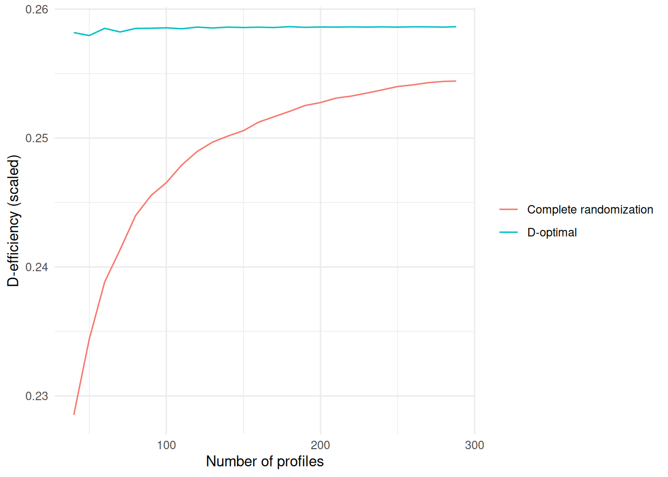
As an exploratory check, we compare a D-optimal selection of profiles against the profiles that complete randomization would draw at the same sample size, restricted to main effects only (the estimand of interest here). At the profile level, using AlgDesign::optFederov (Fedorov algorithm, D-criterion) over the full 288-profile candidate set and the main-effects model ~ Need + Identity + Control + Effort + Reciprocity + Attitude + Sex, we compute the D-efficiency of the optimal design against a benchmark of profiles drawn at random (200 repetitions per grid point) across a grid of sample sizes from 40 to 288 profiles.
library(AlgDesign)library(ggplot2)library(dplyr)set.seed(20260922)# Candidate set: every possible profile (the full 2x3x2x3x2x2x2 = 288 factorial),# one row per profile, one column per attribute. This is the pool optFederov()# will search over -- it cannot propose a profile that isn't in this list.candidates<-gen.factorial( levels =c(2, 3, 2, 3, 2, 2, 2), varNames =c("Need", "Identity", "Control", "Effort", "Reciprocity", "Attitude", "Sex"), factors ="all")# Model to optimize for: main effects only, no interactions (matches the# confirmatory estimator in the Pre-Analysis Plan). model.matrix() turns the# 7 factor columns into the dummy-coded design matrix X; p is its number of# columns (parameters), needed to normalize the D-criterion below.formula_main<-~Need+Identity+Control+Effort+Reciprocity+Attitude+SexX_full<-model.matrix(formula_main, data =candidates)p<-ncol(X_full)# Sample sizes to evaluate, from 40 profiles up to the full 288.n_grid<-seq(40, 288, by =10)if(288%%10!=0)n_grid<-unique(c(n_grid, 288))# Number of random draws averaged per grid point, so the "complete# randomization" benchmark isn't just one noisy draw.n_random_reps<-200# For each candidate sample size N, compute two things and return them as a# one-row data frame (lapply + bind_rows stacks these into one table):results<-lapply(n_grid, function(n){# (a) The D-optimal design of N profiles: optFederov searches the 288-row# candidate set for the N-row subset (with replacement allowed) that# maximizes det(X'X), i.e. is best for estimating the 7 main effects.# nRepeats = 30 restarts the search from different random starting# designs to avoid a local optimum.fed<-optFederov( frml =formula_main, data =candidates, nTrials =n, criterion ="D", nRepeats =30, approximate =FALSE)Xopt<-model.matrix(formula_main, data =fed$design)# D-efficiency, scaled per observation: det(X'X)^(1/p) / n. This puts# designs of different N on a comparable footing -- it is the quantity# that (for a fixed target precision) trades off directly against N.d_opt<-det(t(Xopt)%*%Xopt)^(1/p)/n# (b) The same quantity for N profiles drawn completely at random (with# replacement, exactly as the survey's own randomization would do),# repeated 200 times so we report its expected value rather than one# lucky/unlucky draw.rand_deffs<-replicate(n_random_reps, {idx<-sample(nrow(candidates), n, replace =TRUE)Xr<-model.matrix(formula_main, data =candidates[idx, , drop =FALSE])detXtX<-det(t(Xr)%*%Xr)if(is.na(detXtX)||detXtX<=0)NA_real_elsedetXtX^(1/p)/n})data.frame(N =n, D_optimal =d_opt, D_random =mean(rand_deffs, na.rm =TRUE))})|>bind_rows()|># How much efficiency complete randomization is leaving on the table at# each N, in percentage terms.mutate(gain_pct =100*(D_optimal/D_random-1))# Plot both efficiency curves against N to see how quickly random catches up# to the optimal design.ggplot(results, aes(x =N))+geom_line(aes(y =D_optimal, color ="D-optimal"))+geom_line(aes(y =D_random, color ="Complete randomization"))+labs(x ="Number of profiles", y ="D-efficiency (scaled)", color =NULL)+theme_minimal()
Figure 3.1: D-efficiency (main effects) of a D-optimal profile selection vs. complete randomization, across sample sizes
Walking through what the chunk does: it first builds the candidate set — every one of the 288 possible profiles — since optFederov() can only pick from profiles that exist in this list. It then fixes the model to optimize for, main effects only (formula_main), because efficiency is only meaningful relative to a specific set of parameters. For each sample size in the grid (40 to 288), it runs the Fedorov search to find the best N-profile subset for that model (fed, restarted 30 times to avoid local optima), and computes its per-observation D-efficiency (d_opt). It then computes the same statistic for N profiles drawn completely at random, repeated 200 times so the benchmark reflects the expected efficiency of randomization rather than one draw. Stacking one row per grid point (bind_rows) and adding the percentage gap (gain_pct) gives the results table plotted above.
Across the grid, the D-criterion of the optimal design is essentially flat (0.258–0.2586) regardless of sample size, because with only seven main effects to estimate, the algorithm saturates the available information with very few distinct profiles. Complete randomization converges toward that optimum quickly: the efficiency gap is 13% at N = 40 profiles, falls to 4.9% by N = 100, and is only 1.7% at the full 288-profile factorial. This is consistent with the argument made in the Pre-Analysis Plan: given the small factorial space (288 profiles) and an estimand restricted to main effects, complete randomization is already close to D-optimal, and a formal D-efficient design offers, at most, a modest efficiency gain concentrated at small sample sizes — not a reduction large enough to justify replacing complete randomization, which also has the advantage of preserving marginal-based AMCE identification without fixing the profile set in advance.
Back-of-envelope consequence for sample size. Because \(\text{Var}(\hat\beta) \propto \sigma^2(X'X)^{-1}\), the per-observation D-efficiency computed above trades off directly against N for a fixed target precision: to match the information of the randomized design at size \(N_{\text{random}}\), the D-optimal design only needs \(N_{\text{D-optimal}} \approx N_{\text{random}} / \text{ratio}\), where ratio is D_optimal / D_random at the relevant N. Applying this to the 1,307 respondents required above:
Table 3.1: Back-of-envelope respondents implied by the D-efficiency gain, at selected profile-pool sizes
Profile pool (N)
Efficiency ratio
Respondents (randomization)
Respondents (D-optimal, implied)
40
1.130
1307
1157
100
1.049
1307
1246
288
1.017
1307
1286
The implied saving tracks the efficiency gap directly: on the order of 11% fewer respondents in the most favorable case (a small, 40-profile pool), shrinking to 2% at the full 288-profile factorial — a few hundred respondents at most, not a change of order of magnitude. Two caveats apply. First, this is an approximation: the 1,307 baseline comes from cjpowR’s closed-form AMCE power formula (Schuessler & Freitag, 2020), derived under different assumptions (a Bernoulli-type outcome variance) than the linear-model D-efficiency computed here, so the two are not measuring precision on identical terms — the ratio is a reasonable order-of-magnitude translation, not an exact one. Second, it ignores the respondent fixed effects and cluster-robust standard errors used in the actual estimator (see Analysis considerations), which \((X'X)^{-1}\) alone does not capture. A precise answer would require a Monte Carlo power simulation — fitting the actual respondent-fixed-effects model with clustered SEs to data simulated under each design, across a grid of N — which in turn needs the outcome’s residual variance and intra-respondent correlation. Neither is known yet; calibrating them is one of the stated purposes of the pilot, so a fully rigorous version of this exercise is deferred until pilot data are available.
Pair-level check
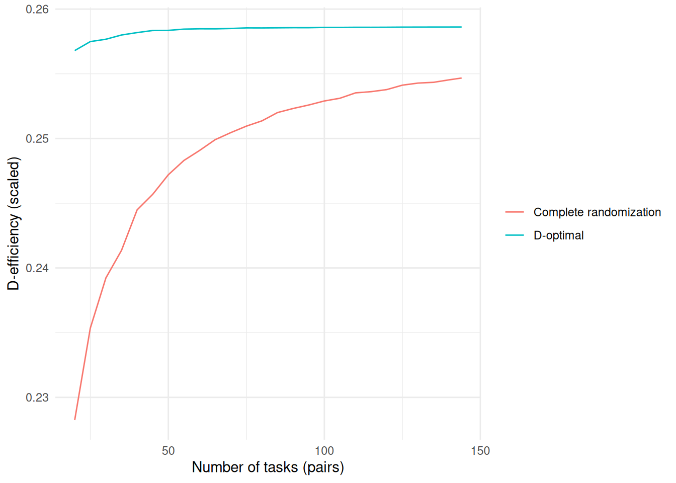
The exercise above optimizes the profile pool, but the unit actually shown to respondents is a task: a pair of two profiles, subject to the restriction that they differ on at least two of the six CARIN/NICER attributes (see Implementation). Because the analysis model has no task-level term — each profile enters the regression as its own row, with only a respondent fixed effect — the information matrix \(X'X\) of the full dataset is just the sum of the two profiles’ individual contributions, regardless of which task paired them. In principle this means pairing does not, by itself, change D-efficiency; what can change it is the restriction, since it rules out some profile combinations and so shrinks the pool the design can be built from. AlgDesign::optFederov does not support this kind of restricted, two-row-per-task candidate set directly, so it is implemented here as a direct pair-level Fedorov-type exchange search: the candidate set is every admissible pair of profiles, and the algorithm swaps one task at a time for a better one whenever doing so raises \(\det(X'X)\) of the full stacked design.
To enumerate the admissible pairs themselves — needed for the survey implementation, not just for the efficiency check — each attribute is now given its actual survey levels and labels, rather than the generic 1, 2, 3 codes used above: Need = dificultad (1) / holgura (2); Identity = chile (1) / venezuela (2) / peru (3); Control = aplico (1) / no aplico (2); Effort = mas (1) / igual (2) / menos (3); Reciprocity = hizo (1) / no hizo (2); Attitude = agradece (1) / merece (2); Sex = mujer (1) / hombre (2). This is a relabeling of the same seven factors, so it does not change the D-efficiency figures below (D-efficiency is invariant to which level is coded as the reference category); what it adds is a labeled candidate set from which the admissible pairs can be listed directly.
library(AlgDesign)library(ggplot2)library(dplyr)library(here)set.seed(20260922)# Candidate profiles, with each attribute's actual survey levels and labels# (rather than generic 1/2/3 codes) so the admissible pairs below are# directly readable/usable for implementation.need_levels<-c("dificultad", "holgura")# 1, 2identity_levels<-c("chile", "venezuela", "peru")# 1, 2, 3control_levels<-c("aplico", "no_aplico")# 1, 2effort_levels<-c("mas", "igual", "menos")# 1, 2, 3reciprocity_levels<-c("hizo", "no_hizo")# 1, 2attitude_levels<-c("agradece", "merece")# 1, 2sex_levels<-c("mujer", "hombre")# 1, 2candidates<-expand.grid( Need =factor(need_levels, levels =need_levels), Identity =factor(identity_levels, levels =identity_levels), Control =factor(control_levels, levels =control_levels), Effort =factor(effort_levels, levels =effort_levels), Reciprocity =factor(reciprocity_levels, levels =reciprocity_levels), Attitude =factor(attitude_levels, levels =attitude_levels), Sex =factor(sex_levels, levels =sex_levels), KEEP.OUT.ATTRS =FALSE)formula_main<-~Need+Identity+Control+Effort+Reciprocity+Attitude+SexX_full<-model.matrix(formula_main, data =candidates)p<-ncol(X_full)# Admissibility matrix: TRUE for profile pairs (i, j) that differ on >= 2 of# the 6 substantive (CARIN/NICER) attributes -- Sex is excluded, as in the# actual survey check. admissible_idx lists every admissible pair once.subst_attrs<-c("Need", "Identity", "Control", "Effort", "Reciprocity", "Attitude")diff_count<-matrix(0L, nrow(candidates), nrow(candidates))for(ainsubst_attrs)diff_count<-diff_count+outer(candidates[[a]], candidates[[a]], FUN ="!=")admissible_mat<-diff_count>=2diag(admissible_mat)<-FALSEadmissible_idx<-which(admissible_mat&upper.tri(admissible_mat), arr.ind =TRUE)n_adm<-nrow(admissible_idx)pct_admissible<-100*n_adm/choose(nrow(candidates), 2)# Materialize every admissible pair as a labeled data frame -- one row per# pair, attributes of profile A and profile B side by side -- and write it# out for use in the survey implementation.profileA<-candidates[admissible_idx[, 1], ]names(profileA)<-paste0(names(profileA), "_A")profileB<-candidates[admissible_idx[, 2], ]names(profileB)<-paste0(names(profileB), "_B")admissible_pairs_df<-cbind(pair_id =seq_len(n_adm), profileA, profileB)rownames(admissible_pairs_df)<-NULLout_dir<-here::here("..", "output", "conjoint-design")dir.create(out_dir, recursive =TRUE, showWarnings =FALSE)write.csv(admissible_pairs_df, file.path(out_dir, "admissible_pairs.csv"), row.names =FALSE)# D-optimal search over n_tasks admissible pairs: starts from a random# selection, then repeatedly tries replacing one task at a time with a# random admissible candidate, keeping the swap only if it raises det(X'X)# of the whole stacked (2*n_tasks-row) design. Restarted n_restarts times# to avoid a local optimum, as optFederov's nRepeats does at the profile level.doptimal_pairs<-function(n_tasks, n_restarts=5, n_sweep=3, n_try=200){best_det<--Inffor(restartinseq_len(n_restarts)){sel<-sample(n_adm, n_tasks, replace =TRUE)pairs<-admissible_idx[sel, , drop =FALSE]contribs<-vector("list", n_tasks)XtX<-matrix(0, p, p)for(kinseq_len(n_tasks)){xi<-X_full[pairs[k, 1], ]; xj<-X_full[pairs[k, 2], ]contribs[[k]]<-outer(xi, xi)+outer(xj, xj)XtX<-XtX+contribs[[k]]}cur_det<-det(XtX)for(sweepinseq_len(n_sweep)){for(kinseq_len(n_tasks)){XtX_wo_k<-XtX-contribs[[k]]cand<-sample(n_adm, n_try)best_local_det<-cur_det; best_local_c<-contribs[[k]]for(cidxincand){ci<-admissible_idx[cidx, 1]; cj<-admissible_idx[cidx, 2]xci<-X_full[ci, ]; xcj<-X_full[cj, ]ck2<-outer(xci, xci)+outer(xcj, xcj)d<-det(XtX_wo_k+ck2)if(d>best_local_det){best_local_det<-d; best_local_c<-ck2}}if(best_local_det>cur_det){XtX<-XtX_wo_k+best_local_ccontribs[[k]]<-best_local_ccur_det<-best_local_det}}}if(cur_det>best_det)best_det<-cur_det}best_det}# Grid of task counts from 20 to 144 (i.e. 40 to 288 profile evaluations,# matching the profile-level grid one-for-one at 2 profiles per task).n_task_grid<-unique(c(seq(20, 144, by =5), 144))n_random_reps<-200results_pair<-lapply(n_task_grid, function(nt){d_opt<-doptimal_pairs(nt)^(1/p)/(2*nt)# Benchmark: n_random_reps sets of nt tasks drawn the way the survey# actually randomizes them -- profiles drawn independently and the pair# kept only if admissible, i.e. a uniform draw from admissible_idx.rand_deffs<-replicate(n_random_reps, {sel<-sample(n_adm, nt, replace =TRUE)pr<-admissible_idx[sel, , drop =FALSE]XtX<-matrix(0, p, p)for(kinseq_len(nt)){xi<-X_full[pr[k, 1], ]; xj<-X_full[pr[k, 2], ]XtX<-XtX+outer(xi, xi)+outer(xj, xj)}detXtX<-det(XtX)if(is.na(detXtX)||detXtX<=0)NA_real_elsedetXtX^(1/p)/(2*nt)})data.frame(N_tasks =nt, D_optimal =d_opt, D_random =mean(rand_deffs, na.rm =TRUE))})|>bind_rows()|>mutate(gain_pct =100*(D_optimal/D_random-1))ggplot(results_pair, aes(x =N_tasks))+geom_line(aes(y =D_optimal, color ="D-optimal"))+geom_line(aes(y =D_random, color ="Complete randomization"))+labs(x ="Number of tasks (pairs)", y ="D-efficiency (scaled)", color =NULL)+theme_minimal()
Figure 3.2: D-efficiency (main effects) of a D-optimal task selection vs. complete randomization under the pairing restriction, across sample sizes
Of the 41,328 possible profile pairs, 38,880 (94.1%) satisfy the restriction, so it rules out only a small corner of the pairing space. Consistent with that, the pair-level curves land almost on top of the profile-level ones: the optimal design is again essentially flat (0.2568–0.2586), and complete randomization under the restriction closes the gap from 12.5% at N = 20 tasks (40 profile evaluations) to 1.5% at N = 144 tasks — practically identical to the unlabeled profile-level run, confirming that the relabeling changes nothing about the design’s statistical properties.
The full candidate list of admissible pairs — 38,880 rows, one per admissible pair, with both profiles’ attribute levels spelled out — is written to output/conjoint-design/admissible_pairs.csv for use in the survey implementation. A preview:
The back-of-envelope translation to respondents (at 5 tasks per respondent, as above) gives the same order of saving as the profile-level check:
Table 3.2: Back-of-envelope respondents implied by the pair-level D-efficiency gain, at selected task-pool sizes
Task pool (N)
Efficiency ratio
Respondents (randomization)
Respondents (D-optimal, implied)
20
1.125
1307
1162
50
1.045
1307
1251
144
1.015
1307
1287
The conclusion is the same as at the profile level, now confirmed under the actual pairing restriction: the restriction itself costs almost nothing in achievable D-efficiency (94% of pairs remain usable), and the ceiling on what a D-efficient task design could save over complete randomization stays in the same modest range, at most on the order of 11% fewer respondents. The same two caveats noted above still apply — the cjpowR baseline is not measured on identical terms, and this ignores respondent fixed effects and clustering — so this remains an exploratory bound, not a substitute for a simulation-based power calculation once pilot data are available.
3.2.4 Implementation
selection of the non-redundant pairs of profiles
restrictions: the design imposes a single restriction, applied to the pair of profiles within a task rather than to individual attributes: the two profiles must differ on at least two of the six CARIN/NICER attributes (need, identity, control, effort, reciprocity, attitude). When a pair is generated, the six substantive attributes are drawn independently and the pair is retained only if it differs on two or more of them, otherwise it is redrawn. Sex is assigned afterward through the applicant’s first name and does not enter the check, so the two profiles may share the same sex or not. The purpose is cognitive: a pair that is identical or differs on only one substantive attribute presents two near-indistinguishable applicants, yielding a task that carries little information about trade-offs.
randomization of attributes order
attention check
inter reliability check
3.2.5 Analysis considerations
3.3 Attitudinal items
This section describes the second component of the survey instrument, complementing the conjoint design presented in the previous section. It first outlines the overall structure of the questionnaire. Then details the batteries of items applied on the pre-pilot survey, describing their conceptual origin, wording, and measurement specifications.
3.3.1 Market justice preferences (MJP)
The “Market Justice Preferences” scale is divided into two parts: the classic items and the new items. The classic scale consists of three questions, which aim to determine the extent to which people consider it fair for access to and the quality of social services—such as education, health care, and pensions—to depend on market criteria. Questions related to education and health care originally come from the International Social Survey Program (1999) and are included in the social inequality module. In this context, the items first appeared in the 1999 version of the ISSP and has been included in all subsequent versions (2009 and 2019). The pensions item came from the Longitudinal Social Study of Chile, a original survey from Chile that was applied between 2016-2023, being available in all waves of the survey.
Both the classic items and the new items can be seen in Table 3.3:
Table 3.3: Market Justice Preferences items
N
Model
Phrasing english
Item english
Phrasing spanish
Item spanish
1
MJP Classic
NA
It is fair that in Chile, high-income individuals have access to better health care than those with lower incomes
NA
Es justo que en Chile las personas de altos ingresos puedan acceder a una mejor atención de salud que las personas con ingresos más bajos
2
MJP Classic
NA
It is fair that in Chile, high-income individuals have access to better education than those with lower incomes
NA
Es justo que en Chile las personas de altos ingresos tengan una mejor educación para sus hijos que las personas con ingresos más bajos
3
MJP Classic
NA
It is fair that high-income individuals in Chile receive better pensions than those with lower incomes
NA
Es justo que en Chile las personas de altos ingresos tengan mejores pensiones que las personas con ingresos más bajos
The classic items (1-3) are measured using a Likert scale ranging from “disagree” to “agree,” where (1) is “strongly disagree” (muy en desacuerdo) and (5) is “strongly agree” (muy de acuerdo).
3.3.2 MJP Reflexive
This survey draws on the Market Justice Preferences measurement framework with the aim of expanding the measurement of this concept. To this end, the research team developed a set of items designed to capture respondents’ perceptions of market justice from two perspectives: (1) their personal access to social services and (2) their children’s access to social services (see (tbl.mjpr?)).
Table 3.4: MJP Reflexive items
N
Model
Phrasing english
Item english
Phrasing spanish
Item spanish
1
MJP Reflexive
NA
It’s fair that I have access to better health care if I can afford it
NA
Es justo que yo tenga acceso a una mejor salud si puedo pagar por ello
2
MJP Reflexive
NA
It’s fair that I have access to a better education if I can afford it
NA
Es justo que yo tenga acceso a una mejor educación si puedo pagar por ello
3
MJP Reflexive
NA
It’s fair that I have access to a better pension if I can afford it
NA
Es justo que yo tenga acceso a mejor pensión si puedo pagar por ello
4
MJP Reflexive
NA
It’s okay for my children to have access to better health care than other children if I can afford it
NA
Está bien que mis hijos/as tengan acceso a una mejor salud que otros niños si es que puedo pagar por ello
5
MJP Reflexive
NA
It’s okay for my children to have access to a better education than other children if I can afford it
NA
Está bien que mis hijos/as tengan acceso a una mejor educación que otros niños si es que puedo pagar por ello
Items referring to personal circumstances (me) are measured using a Likert scale, where (1) is “Strongly disagree” (Muy en desacuerdo) and (5) is “Strongly agree” (Muy de acuerdo). Meanwhile, the items referring to the children’s situation (my children) are measured on a Likert scale ranging from “Very unfair” (Muy injusto) (1) to “Very fair” (Muy justo) (5).
3.3.3 MJP Over time
The MJP Over Time questions aim to capture respondents’ perceptions of market fairness regarding access to social services in comparative temporal terms (see Table 3.5). Thus, two sets of items were created: the first set aims to measure the perceived level of inequality regarding social services, while the second set aims to measure how much inequality in access to social services has changed over the past 10 years.
Table 3.5: MJP Over time items
N
Model
Phrasing english
Item english
Phrasing spanish
Item spanish
1
MJP Time
To what extent do you agree or disagree with the following statements?
Access to health care is unequal in Chile
¿En qué medida está de acuerdo o en desacuerdo con las siguientes afirmaciones?
El acceso a la salud es desigual en Chile
2
MJP Time
To what extent do you agree or disagree with the following statements?
Access to education is unequal in Chile
¿En qué medida está de acuerdo o en desacuerdo con las siguientes afirmaciones?
El acceso a la educación es desigual en Chile
3
MJP Time
To what extent do you agree or disagree with the following statements?
Pensions are unequal in Chile
¿En qué medida está de acuerdo o en desacuerdo con las siguientes afirmaciones?
Las pensiones son desiguales en Chile
4
MJP Time
And thinking back 10 years, do you think access to the following services among those with higher and lower incomes has become…?
Health care
Y pensando hace 10 años atrás, ¿usted cree que el acceso a los siguientes servicios entre quienes tienes más y menores ingresos se ha vuelto…?
Salud
5
MJP Time
And thinking back 10 years, do you think access to the following services among those with higher and lower incomes has become…?
Education
Y pensando hace 10 años atrás, ¿usted cree que el acceso a los siguientes servicios entre quienes tienes más y menores ingresos se ha vuelto…?
Educación
6
MJP Time
And thinking back 10 years, do you think access to the following services among those with higher and lower incomes has become…?
Pensions
Y pensando hace 10 años atrás, ¿usted cree que el acceso a los siguientes servicios entre quienes tienes más y menores ingresos se ha vuelto…?
Pensiones
The first three items are measured using a five-point Likert scale ranging from “Very unequal” (Muy desigual) (1) to “Not at all unequal” (Nada desigual) (5). The last three items, meanwhile, are measured using a five-point Likert scale ranging from “Much more unequal” (Mucho más desigual) (1) to “Much less unequal” (Mucho menos desigual) (5).
3.3.4 Commodification of social services
The research team first administered a series of questions designed to measure the extent to which it is acceptable for social services to operate (or not) according to a logic of commodification. In this context, the first two items seek to measure the degree of acceptance of social services being managed by private entities, while the last three items present a different scenario: measuring the degree of agreement that social services should not operate based on ability to pay, implying that there should be a single quality standard for all users (for better understanding see Table 3.6).
Table 3.6: Commodification of social services items
N
Model
Phrasing english
Item english
Phrasing spanish
Item spanish
1
Service commodification
NA
It’s fine for public hospitals to be managed by private entities if they are able to provide better service
NA
Está bien que los hospitales públicos sean administrados por privados si ellos son capaces de brindar un mejor servicio
2
Service commodification
NA
It’s fine for public high schools to be run by private entities if they are able to provide a better service
NA
Está bien que los liceos públicos sean administrados por privados si ellos son capaces de brindar un mejor servicio
3
Service commodification
NA
The quality of the health care system should be the same for everyone, even if that means my family can’t afford better services.
NA
La calidad del sistema de salud debería ser igual para todos aunque esto signifique que mi familila no pueda pagar por mejores servicios
4
Service commodification
NA
Education should be of equal quality for everyone, even if that means I can’t afford a better one for my family
NA
La educación debería ser de igual calidad para todos aunque eso me impida pagar por una mejor para mi familia
5
Service commodification
NA
Pensions should be more equitable, even if that means I receive a pension similar to those who contributed less than I did
NA
Las pensiones deberían ser más igualitarias, aunque eso signifique que yo reciba una pensión similar a quienes aportaron menos que yo
The five items are measured using a Likert scale, where (1) is “Strongly Disagree” and (5) is “Strongly Agree.”
3.3.5 Profit of social services
This set of questions contains three items designed to measure perceptions of fairness regarding the use of social services to generate monetary profits. The research team therefore proposed the same basic question but varied the social service, choosing from: (1) Health, (2) Education, and (3) Pensions (see Table 3.7).
Table 3.7: Profit of social services items
N
Model
Phrasing english
Item english
Phrasing spanish
Item spanish
1
Profit
How fair or unfair do you think it is for private companies to make a profit by managing…
Health care
Qué tan justo o injusto le parece que empresas privadas obtengan ganancias monetarias administrando…
Salud
2
Profit
How fair or unfair do you think it is for private companies to make a profit by managing…
Education
Qué tan justo o injusto le parece que empresas privadas obtengan ganancias monetarias administrando…
Educación
3
Profit
How fair or unfair do you think it is for private companies to make a profit by managing…
Pensions
Qué tan justo o injusto le parece que empresas privadas obtengan ganancias monetarias administrando…
Pensiones
All items in this battery are measured using a Likert scale, where (1) is “Very unfair” (Muy injusto) and (5) is “Very fair” (Muy justo).
3.3.6 Investment in social services
These questions are based on research by Busemeyer et al. (2018), which includes a series of items designed to measure investment preferences regarding public policies. For this survey, three of the original items were used, and two new items were added, relating to daycare centers and roads (see Table 3.8).
Table 3.8: Investment in social services items
N
Model
Phrasing english
Item english
Phrasing spanish
Item spanish
1
Policy spending
Below are some areas of government activity. Please indicate whether you would like to see public spending increased or decreased in each of these areas. Keep in mind that “more” or “much more” could mean a tax increase.
Health care
A continuación, se mencionan algunos ámbitos de la actividad gubernamental. Por favor, señale si le gustaría que se aumentara o se redujera el gasto público en cada uno de ellos. Tenga en cuenta que «más» o «mucho más» podría implicar un alza de impuestos.
Salud
2
Policy spending
Below are some areas of government activity. Please indicate whether you would like to see public spending increased or decreased in each of these areas. Keep in mind that “more” or “much more” could mean a tax increase.
Education
A continuación, se mencionan algunos ámbitos de la actividad gubernamental. Por favor, señale si le gustaría que se aumentara o se redujera el gasto público en cada uno de ellos. Tenga en cuenta que «más» o «mucho más» podría implicar un alza de impuestos.
Educación
3
Policy spending
Below are some areas of government activity. Please indicate whether you would like to see public spending increased or decreased in each of these areas. Keep in mind that “more” or “much more” could mean a tax increase.
Pensions
A continuación, se mencionan algunos ámbitos de la actividad gubernamental. Por favor, señale si le gustaría que se aumentara o se redujera el gasto público en cada uno de ellos. Tenga en cuenta que «más» o «mucho más» podría implicar un alza de impuestos.
Pensiones
4
Policy spending
Below are some areas of government activity. Please indicate whether you would like to see public spending increased or decreased in each of these areas. Keep in mind that “more” or “much more” could mean a tax increase.
Childcare
A continuación, se mencionan algunos ámbitos de la actividad gubernamental. Por favor, señale si le gustaría que se aumentara o se redujera el gasto público en cada uno de ellos. Tenga en cuenta que «más» o «mucho más» podría implicar un alza de impuestos.
Cuidado de niños
5
Policy spending
Below are some areas of government activity. Please indicate whether you would like to see public spending increased or decreased in each of these areas. Keep in mind that “more” or “much more” could mean a tax increase.
Roads
A continuación, se mencionan algunos ámbitos de la actividad gubernamental. Por favor, señale si le gustaría que se aumentara o se redujera el gasto público en cada uno de ellos. Tenga en cuenta que «más» o «mucho más» podría implicar un alza de impuestos.
Carreteras
The five items in the battery are measured using a Likert scale, where (1) is “Much less spending” (Mucho menos gasto) and (5) is “Much more spending” (Mucho más gasto).
3.3.7 Deservingness
The deservingness scale is based on the conceptual and empirically validated proposal by Meuleman et al. (2020), which allows for an empirical study of the normative criteria that citizens apply to determine who is eligible for social protection. The framework is built upon the operationalization of five central concepts:
Control: Refers to the perception of personal responsibility in the face of a situation of need.
Attitude: Assesses the beneficiary’s disposition toward society and their gratitude for the assistance received.
Reciprocity: Considers the beneficiary’s past or future contribution to the system, which implies an expectation of a return for the assistance people receive.
Identity: Assesses the moral boundaries of the community regarding its willingness to benefit another.
Need: Focuses on the urgency and severity of the beneficiary’s situation. In this case, need is distinguished from control because it refers to conditions that are beyond an individual’s control.
In addition, this survey includes the “effort” dimension based on the proposal by Knotz et al. (2022), who defines effort as the beneficiary’s active and present agency aimed at overcoming their situation of vulnerability or contributing in some way to society at the time they receive support. Based on these two models for measuring deservingness, this survey includes the following items (see Table 3.9):
Table 3.9: Deservingness scale items
Model
Dimension
Item english
Item spanish
CARIN
Control
People who fall into poverty because of their own mistakes should still have the right to receive support from the government
Las personas que caen en la pobreza por sus propios errores deberían igualmente tener derecho a recibir apoyo del Estado
CARIN
Control
People who are responsible for their own problems also deserve to receive social benefits
Quienes son responsables de sus propios problemas igualmente merecen recibir beneficios sociales
CARIN
Control
The government should help people regardless of whether their situation was caused by their own decisions or by external factors
El Estado debería ayudar a las personas independientemente de si su situación fue causada por decisiones propias o por factores externos
CARIN
Attitude
People who receive government benefits should show more gratitude for the assistance they receive
Las personas que reciben beneficios del Estado deberían mostrar más gratitud por la ayuda que reciben
CARIN
Attitude
It is acceptable for people who receive government assistance to express their dissatisfaction with the terms of their benefits
Está bien que las personas que reciben apoyo del Estado puedan expresar su descontento con las condiciones de los beneficios
CARIN
Reciprocity
Social benefits should be reserved for those who have previously contributed to the system, for example, by making contributions or paying taxes
Los beneficios sociales deberían estar reservados para quienes han contribuido previamente al sistema, por ejemplo cotizando o pagando impuestos
CARIN
Reciprocity
It is not fair that people who have never contributed to the system receive the same benefits as those who have.
No es justo que personas que nunca han contribuido al sistema reciban los mismos beneficios que quienes sí lo han hecho
CARIN
Reciprocity
Those who have worked and contributed to the system for a longer period of time deserve better social benefits than those who have contributed little or nothing
Quienes han trabajado y aportado al sistema durante más tiempo merecen mejores beneficios sociales que quienes han contribuido poco o nada
CARIN
Reciprocity
Access to social benefits should be the same for everyone, regardless of whether or not they have made contributions in the past
El acceso a los beneficios sociales debería ser el mismo para todos, independientemente de si han cotizado o no en el pasado
CARIN
Identity
When allocating social benefits, people born in Chile should be given priority over those who came from other countries
Al momento de asignar beneficios sociales, las personas nacidas en Chile deberían tener prioridad por sobre quienes llegaron de otros países
CARIN
Identity
Migrants should have access to the same social benefits as Chileans
Los migrantes deberían tener acceso a los mismos beneficios sociales que los chilenos
CARIN
Identity
Only those who have been living in Chile for several years should be eligible for the government’s social protection programs
Solo quienes llevan varios años viviendo en Chile deberían poder acceder a los programas de protección social del Estado
CARIN
Need
Social benefits should be reserved exclusively for those living in actual poverty
Los beneficios sociales deberían estar reservados exclusivamente para quienes viven en situación de pobreza real
CARIN
Need
People who have sufficient financial resources of their own should not receive government assistance
Las personas que tienen suficientes recursos económicos propios no deberían recibir apoyo del Estado
CARIN
Need
Only those in extreme need should be eligible for social benefits
Solo quienes se encuentran en situación de extrema necesidad deberían poder acceder a los beneficios sociales
NICER
Effort
People who receive social benefits should be actively doing something to improve their situation, such as looking for work or getting training
Las personas que reciben beneficios sociales deberían estar haciendo algo activamente para mejorar su situación, como buscar trabajo o capacitarse
NICER
Effort
People who receive government assistance but make no effort to get ahead deserve less support than those who do try
Quienes reciben ayuda del Estado pero no hacen ningún esfuerzo por salir adelante merecen menos apoyo que quienes sí lo intentan
NICER
Effort
The government should support people even if they are not making any visible effort to change their situation
El Estado debería apoyar a las personas aunque no estén haciendo ningún esfuerzo visible por cambiar su situación
NICER
Effort
It is reasonable for the duration of a social benefit to depend on the effort the person is making to no longer need it
Es razonable que la duración de un beneficio social dependa del esfuerzo que está haciendo la persona para dejar de necesitarlo
NICER
Effort
It doesn’t matter whether someone is looking for a job or not: if they need help, the government should provide it regardless
No importa si alguien está buscando trabajo o no: si necesita ayuda, el Estado debería dársela igual
The items are measured using a Likert scale ranging from “disagree” to “agree,” where (1) is “strongly disagree” (muy en desacuerdo) and (5) is “strongly agree” (muy de acuerdo).
3.3.8 Meritocracy
The meritocracy scale is based on a conceptual framework designed by Castillo et al. (2023), which presents a multidimensional model for measuring meritocratic beliefs. This model distinguishes, first, between perceptions and preferences, where the former refers to the way people view the world, while the latter refers to how the world should function. Second, the model distinguishes between meritocratic and privilege-based perceptions and preferences; meritocratic factors relate to effort and talent, while the privilege factor considers inherited conditions such as family wealth and connections. This instrument was first implemented in a survey conducted between 2019 and 2020 as part of the FONDECYT Regular project “The Moral Economy of Meritocracy and Redistributive Preferences”. Subsequently, this set of questions has been used in surveys targeting student and adult populations.
To better illustrate the items that make up the scale, the following table is provided (see Table 3.10):
Table 3.10: Meritocracy scale items
Dimensions
Factor
Item english
Item spanish
Perception
Meritocratic
In Chile people are rewarded for their efforts
En Chile las personas son recompensadas por sus esfuerzos
Perception
Meritocratic
In Chile people are rewarded for their intelligence and ability
En Chile las personas son recompensadas por su inteligencia y habilidad
Perception
Privilege
In Chile those with wealthy parents do much better in life
En Chile a quienes tienen padres ricos les va mucho mejor en la vida
Perception
Privilege
In Chile those with good contacts do much better in life
En Chile a quienes tienen buenos contactos les va mejor en la vida
Preference
Meritocratic
Those who work harder should reap greater rewards than those who work less hard
Quienes más se esfuerzan deberían obtener mayores recompensas que quienes se esfuerzan menos
Preference
Meritocratic
Those with more talent should reap greater rewards than those with less talent
Quienes poseen más talento deberían obtener mayores recompensas que quienes poseen menos talento
Preference
Privilege
It is good that those who have rich parents do better in life
Está bien que quienes tengan padres ricos les vaya mejor en la vida
Preference
Privilege
It is good that those who have good contacts do better in life
Está bien que quienes tengan buenos contactos les vaya mejor en la vida
Each item on the scale is measured using a four-point agreement-disagreement scale, where (1) indicates “strongly disagree” and (4) indicates “strongly agree.” It is worth noting that this scale does not include any intermediate categories.
3.3.9 Anti-Neoliberalism
The following questions were taken from the Anti-Neoliberal Attitudes Scale proposed by Grzanka et al. (2020) in their paper titled “Measuring Neoliberalism: Development and Initial Validation of a Scale of Anti-Neoliberal Attitudes”. In the study, this scale was tested, and its metric consistency was verified for use. The team analyzed the scale and decided to include in the pre-pilot only those items that were thematically relevant to the survey, selecting just 4 items out of a total of 6 that make up one of the scale’s factors (see Table 3.11).
Table 3.11: Neoliberalism items
Model
Item english
Item spanish
Neoliberalism
The government should provide the entire population with basic services such as health care and legal assistance free of charge
El Gobierno debería proporcionar a toda la población servicios básicos como la asistencia sanitaria y la asistencia jurídica de forma gratuita
Neoliberalism
If the government has to increase its debt to help people, it should do so
Si el Gobierno tiene que aumentar su deuda para ayudar a la gente, debería hacerlo
Neoliberalism
Society should provide free resources and services to people who cannot afford them
La sociedad debería proporcionar recursos y servicios gratuitos a las personas que no pueden permitírselos
Neoliberalism
People with higher incomes should pay more taxes than those with lower incomes
Las personas con ingresos más elevados deberían pagar más impuestos que las que tienen ingresos más bajos
The four items are measured using a Likert scale ranging from “disagree” to “agree,” where (1) is “strongly disagree” (muy en desacuerdo) and (5) is “strongly agree” (muy de acuerdo).
3.3.10 Socioeconomic concern items
This final scale was created by the project team with the goal of capturing people’s perceptions regarding their personal financial concerns. Since these questions were proposed specifically for this questionnaire, they have not been included in previous surveys. The questions can be viewed at Table 3.12
Table 3.12: Socioeconomic concern items
Model
Phrasing english
Item english
Phrasing spanish
Item spanish
Additional
Which of the following statements best describes your current situation, considering your total current income?
¿Cuál de las siguientes afirmaciones describe mejor su situación actual, considerando el total de ingresos que tiene actualmente?
Additional
How often do you feel worried about the following situations?
May my financial situation get worse in the coming years.
¿Con qué frecuencia se siente preocupado por las siguientes situaciones?
Que mi situación financiera empeore los próximos años.
Additional
How often do you feel worried about the following situations?
To become unemployed
¿Con qué frecuencia se siente preocupado por las siguientes situaciones?
Quedar desempleado
Additional
How often do you feel worried about the following situations?
That my children and future generations will have a much harder time
¿Con qué frecuencia se siente preocupado por las siguientes situaciones?
Que mis hijos/as y las próximas generaciones lo tendrán mucho más difícil
The first question includes the following response categories: (1) We don’t have enough, we have major problems; (2) We barely make ends meet by cutting back on expenses; (3) We have just enough and can treat ourselves to a few things without any major problems; (4) We have plenty, we can even save some money.
The other three questions are measured using a five-point Likert scale, where (1) means “never” and (5) means “often.”
3.3.11 Socio-economic characterization
The demographic questions included in the survey are the standard ones used in questionnaires to gather demographic and socioeconomic information about respondents. One innovation in the profiling questionnaire is the last two questions in the Table 3.13 section, which are designed to identify respondents’ background regarding the social services they receive, which aligns with a “market justice” type of profiling.
Each question has a set of answer categories related to the topic. For instance, The question regarding the device used to complete the survey offers only the categories “cell phone,” “tablet,” and “computer,” since it is an online survey. On the other hand, “Income” contains 10 answer categories, ranging from “Up to $344,999” to “$3,100,000 or more” per month.
Table 3.13: Characterization items
Model
Item english
Item spanish
Characterization
Which device are you using to take this survey?
¿Desde qué dispositivo responde esta encuesta?
Characterization
What is their gender?
¿Cuál es su sexo?
Characterization
What year were you born?
¿En qué año nació?
Characterization
What is the highest level of education you have completed? If you are currently enrolled in school, list the highest degree you have earned.
¿Cuál es el nivel educativo más alto que ha completado? Si actualmente está estudiando, use el grado más alto que haya obtenido.
Characterization
What is your gender identity?
¿Cuál es su identidad de género?
Characterization
What is your annual household income (from all sources) before taxes and other deductions?
¿Cuál es su ingreso anual del hogar (de todas las fuentes) antes de impuestos y otras deducciones?
Characterization
What health insurance plan do you have?
¿Qué plan de salud tiene?
Characterization
What kind of school did you attend?
¿En qué tipo de colegio estudió?
Bansak, K., Hainmueller, J., Hopkins, D. J., & Yamamoto, T. (2021). Conjoint Survey Experiments. In J. Druckman & D. P. Green (Eds.), Advances in Experimental Political Science (1st ed., pp. 19–41). Cambridge University Press. https://doi.org/10.1017/9781108777919.004
Busemeyer, M. R., Garritzmann, J. L., Neimanns, E., & Nezi, R. (2018). Investing in education in Europe: Evidence from a new survey of public opinion. Journal of European Social Policy, 28(1), 34–54. https://doi.org/10.1177/0958928717700562
Castillo, J. C., Iturra, J., Maldonado, L., Atria, J., & Meneses, F. (2023). A Multidimensional Approach for Measuring Meritocratic Beliefs: Advantages, Limitations and Alternatives to the ISSP Social Inequality Survey. International Journal of Sociology, 53(6), 448–472. https://doi.org/10.1080/00207659.2023.2274712
Gilgen, S. (2022). Disentangling Justice: Needs, Equality or Merit? On the Situation-Dependency of Distributive Justice (1. Auflage). Baden-Baden: Nomos Verlagsgesellschaft mbH & Co. KG. https://doi.org/10.5771/9783748926955
Grzanka, P. R., Miles, J. R., Spengler, E. S., Arnett, J. E., & Pruett, J. (2020). Measuring Neoliberalism: Development and Initial Validation of a Scale of Anti-Neoliberal Attitudes. Social Justice Research, 33(1), 44–80. https://doi.org/10.1007/s11211-019-00339-3
Hainmueller, J., Hopkins, D. J., & Yamamoto, T. (2014). Causal Inference in Conjoint Analysis: Understanding Multidimensional Choices via Stated Preference Experiments. Political Analysis, 22(1), 1–30. https://doi.org/10.1093/pan/mpt024
Knotz, C. M., Gandenberger, M. K., Fossati, F., & Bonoli, G. (2022). A Recast Framework for Welfare Deservingness Perceptions. Social Indicators Research, 159(3), 927–943. https://doi.org/10.1007/s11205-021-02774-9
Meuleman, B., Roosma, F., & Abts, K. (2020). Welfare deservingness opinions from heuristic to measurable concept: The CARIN deservingness principles scale. Social Science Research, 85, 102352. https://doi.org/10.1016/j.ssresearch.2019.102352
Oorschot, W. V. (2000). Who should get what, and why? On deservingness criteria and the conditionality of solidarity among the public. Policy & Politics, 28(1), 33–48. https://doi.org/10.1332/0305573002500811