The distributive conjoint’s identification argument (see Questionnaire design A: Distributive Conjoint Survey Experiment, Causal identification) rests on complete, independent randomization of attribute levels: every attribute is drawn uniformly and independently of every other attribute and of the competing profile, subject only to a pairwise restriction that the two profiles in a task differ on at least two attributes. A natural concern is whether this restriction, or any implementation detail of the randomizer, inadvertently introduces correlation between attributes, which would threaten the orthogonality the AMCE estimator assumes.
This appendix answers that concern empirically rather than asserting it. It simulates data using the exact randomization procedure implemented in surveys/pre-piloto/sin_comentarios/app.R (the pre-pilot Shiny/surveydown app), and then checks (a) how densely the design space is covered and (b) whether attribute levels are correlated with one another, both within a profile and across the two profiles of a task.
9.2.2 Design parameters, as implemented in app.R
The parameters below are read directly from build_default_conjoint_design() and make_cbc_table() in app.R, not reconstructed from the design write-up, so that the simulation cannot silently drift from what the app actually does.
Seven attributes. Six are explicit rows in the profile table — need, identity, control, effort, reciprocity, attitude — plus applicant sex, signaled only through a first name (never an explicit row).
Levels and marginal probabilities. Every level within an attribute is drawn with sample(lvls, 1), i.e. uniformly: 1/2 for the five binary attributes (need, control, reciprocity, attitude, sex) and 1/3 for the two three-level attributes (identity, effort). The exact level strings coded in niveles are reproduced in Table 9.1 below.
Pairwise restriction.generate_pair() draws the two profiles’ six explicit attributes (identity/need/control/effort/reciprocity/attitude — not sex) independently and redraws the whole pair — both profiles, all six attributes — whenever they differ on fewer than min_diff = 2 attributes. This is a rejection sampler operating on the joint distribution of the pair, not a constraint on any single attribute’s marginal.
Attribute display order / NICERA code. Once per respondent, sample() draws a random permutation of the six explicit attribute names; this order is held constant across that respondent’s six tasks and is persisted as a 6-letter code (Need, Identity, Control, Effort, Reciprocity, Attitude) via attr_code. Sex is not part of this code — it always occupies the profile header, never a randomized row position.
Six tasks, two profiles per task, one respondent draws one respondent-level design row (respID) from the pre-generated design table, or, when the newer profile columns are absent, falls back to build_default_conjoint_design() — the function reproduced here.
niveles<-list( need =c("Dificultad", "Holgura"), identity =c("Chile", "Venezuela", "Perú"), control =c("Postuló a otras becas pero no obtuvo financiamiento","No alcanzó a postular a tiempo a otras becas"), effort =c("Más que sus compañeros","Igual que sus compañeros","Menos que sus compañeros"), reciprocity =c("Ha hecho voluntariado", "No ha hecho voluntariado"), attitude =c("Una ayuda que agradece", "Algo que se merece"))attr_names<-names(niveles)n_levels<-lengths(niveles)library(kableExtra)data.frame( Attribute =attr_names, N_levels =n_levels, P_level =paste0("1/", n_levels), Levels =sapply(niveles, paste, collapse =" | "))|>kbl(row.names =FALSE, col.names =c("Attribute", "N levels", "P(level)", "Levels (as coded)"))|>kable_styling(bootstrap_options =c("striped", "condensed"), full_width =TRUE)
Table 9.1: Attributes and levels exactly as coded in app.R’s niveles list
Attribute
N levels
P(level)
Levels (as coded)
need
2
1/2
Dificultad | Holgura
identity
3
1/3
Chile | Venezuela | Perú
control
2
1/2
Postuló a otras becas pero no obtuvo financiamiento | No alcanzó a postular a tiempo a otras becas
effort
3
1/3
Más que sus compañeros | Igual que sus compañeros | Menos que sus compañeros
reciprocity
2
1/2
Ha hecho voluntariado | No ha hecho voluntariado
attitude
2
1/2
Una ayuda que agradece | Algo que se merece
Sex is not in niveles (it is generated separately), so it is added here only for reference: two levels, drawn uniformly, from an 8-name pool per sex (male_names, female_names in app.R).
With seven attributes at these level counts, the profile space has \(2 \times 3 \times 2 \times 3 \times 2 \times 2 \times 2 = 288\) unique combinations, matching the main design chapter.
9.2.3 Step 1 — Simulating respondents
The simulation targets \(N = 4{,}000\) respondents, 6 tasks each, 2 profiles per task. Pair generation replicates generate_pair() exactly (independent uniform draw per attribute for each profile, redraw the whole pair if it differs on fewer than 2 of the six explicit attributes), implemented here as a vectorized rejection sampler for speed rather than the app’s per-pair repeat loop; the acceptance rule is identical, only the batching differs.
if(!require("pacman"))install.packages("pacman")pacman::p_load(dplyr,tidyr, purrr,tibble,jsonlite,stringr,psych,corrplot)set.seed(2026)N<-4000n_tasks<-6n_pairs<-N*n_tasks# one pair of profiles per task# Vectorized version of generate_pair(): draw a batch of candidate pairs,# keep only those differing on >= 2 of the 6 explicit attributes, repeat# until enough admissible pairs have been collected.gen_batch<-function(n){m1<-sapply(n_levels, function(L)sample.int(L, n, replace =TRUE))m2<-sapply(n_levels, function(L)sample.int(L, n, replace =TRUE))keep<-rowSums(m1!=m2)>=2list(m1 =m1[keep, , drop =FALSE], m2 =m2[keep, , drop =FALSE])}acc1<-matrix(nrow =0, ncol =6)acc2<-acc1while(nrow(acc1)<n_pairs){batch<-gen_batch(ceiling((n_pairs-nrow(acc1))*1.15)+10)acc1<-rbind(acc1, batch$m1)acc2<-rbind(acc2, batch$m2)}acc1<-acc1[seq_len(n_pairs), ]acc2<-acc2[seq_len(n_pairs), ]colnames(acc1)<-attr_namescolnames(acc2)<-attr_namesstopifnot(min(rowSums(acc1!=acc2))>=2)# restriction holds for every task# Map integer level codes back to the label strings coded in nivelesto_labels<-function(m){as.data.frame(lapply(attr_names, function(a)niveles[[a]][m[, a]]), col.names =attr_names, stringsAsFactors =FALSE)}lab1<-to_labels(acc1)lab2<-to_labels(acc2)# Sex/name: independent per profile-slot, exactly as in make_cbc_table()sex_draw<-function(n){is_male<-runif(n)<0.5nm<-character(n)nm[is_male]<-sample(male_names, sum(is_male), replace =TRUE)nm[!is_male]<-sample(female_names, sum(!is_male), replace =TRUE)nm}lab1$nombre<-sex_draw(n_pairs)lab2$nombre<-sex_draw(n_pairs)session_id<-rep(seq_len(N), each =n_tasks)task_id<-rep(seq_len(n_tasks), times =N)lab1$session_id<-session_id; lab1$task_id<-task_idlab2$session_id<-session_id; lab2$task_id<-task_id# Attribute display order per respondent -> NICERA code, exactly as in app.Rattr_order_mat<-t(replicate(N, sample(attr_names)))nicera_code<-apply(attr_order_mat, 1, function(o)paste(attr_code[o], collapse =""))
9.2.4 Step 2 — Assembling the simulated cbc_profiles database
app.R stores one JSON blob per respondent (cbc_profiles) with the six tasks nested under keys q1–q6, each holding the two alternatives under a1/a2, each alternative holding the six attribute values plus nombre. It also stores the display order as cbc_attr_order (the NICERA code) and — via surveydown’s own input persistence — one slider answer per task (cbc_q1-cbc_q6).
The slider/share values are not simulated from any effect model here: this appendix checks randomization structure, not treatment effects.
build_json_for_session<-function(df1, df2){tasks<-vector("list", n_tasks)for(tinseq_len(n_tasks)){tasks[[t]]<-list( a1 =c(as.list(df1[t, attr_names, drop =FALSE]), nombre =df1$nombre[t]), a2 =c(as.list(df2[t, attr_names, drop =FALSE]), nombre =df2$nombre[t]))}names(tasks)<-paste0("q", seq_len(n_tasks))as.character(toJSON(tasks, auto_unbox =TRUE))}split1<-split(lab1, lab1$session_id)split2<-split(lab2, lab2$session_id)profiles_json<-map2_chr(split1, split2, build_json_for_session)# Placeholder share: a random even split per task, complementary by# construction (share_a1 + share_a2 = 100) so the fixed-sum shape of the# real outcome is preserved structurally. NOT used to estimate anything.share_a1<-matrix(runif(n_pairs, 0, 100), nrow =N, ncol =n_tasks, byrow =TRUE)sim_db<-tibble( session_id =as.integer(names(split1)), cbc_attr_order =nicera_code, cbc_profiles =profiles_json)|>bind_cols(as.data.frame(share_a1)|>setNames(paste0("cbc_q", seq_len(n_tasks))))glimpse(sim_db[1, ])
sim_db now has the same shape as the real response table would.
9.2.5 Step 3 — Reshape to long format
This is the pipeline that will be applied to the real pilot export: parse each respondent’s cbc_profiles JSON, unnest tasks and alternatives into one row per session_id × task × altID, and recover sex from nombre via the same name pools app.R draws from.
Postuló a otras becas pero no obtuvo financiamiento
Igual que sus compañeros
No ha hecho voluntariado
Una ayuda que agradece
female
1
1
2
Dificultad
Chile
Postuló a otras becas pero no obtuvo financiamiento
Igual que sus compañeros
Ha hecho voluntariado
Una ayuda que agradece
female
1
2
1
Dificultad
Chile
No alcanzó a postular a tiempo a otras becas
Más que sus compañeros
Ha hecho voluntariado
Algo que se merece
male
1
2
2
Holgura
Perú
No alcanzó a postular a tiempo a otras becas
Igual que sus compañeros
Ha hecho voluntariado
Una ayuda que agradece
female
long_df has 48000 rows — 4000 respondents × 6 tasks × 2 alternatives — one row per presented profile, with the seven attributes as columns. This is the table format the pilot analysis (and the AMCE models in the main design chapter) will be estimated on.
Postuló a otras becas pero no obtuvo financiamiento
24152
effort
Igual que sus compañeros
15943
effort
Menos que sus compañeros
16180
effort
Más que sus compañeros
15877
reciprocity
Ha hecho voluntariado
24039
reciprocity
No ha hecho voluntariado
23961
attitude
Algo que se merece
23930
attitude
Una ayuda que agradece
24070
sex
female
23811
sex
male
24189
Every level of every attribute lands close to its expected count (\(N \times 6 \times 2\) divided by the number of levels), consistent with uniform, independent draws.
9.2.7 Orthogonality: correlation matrix
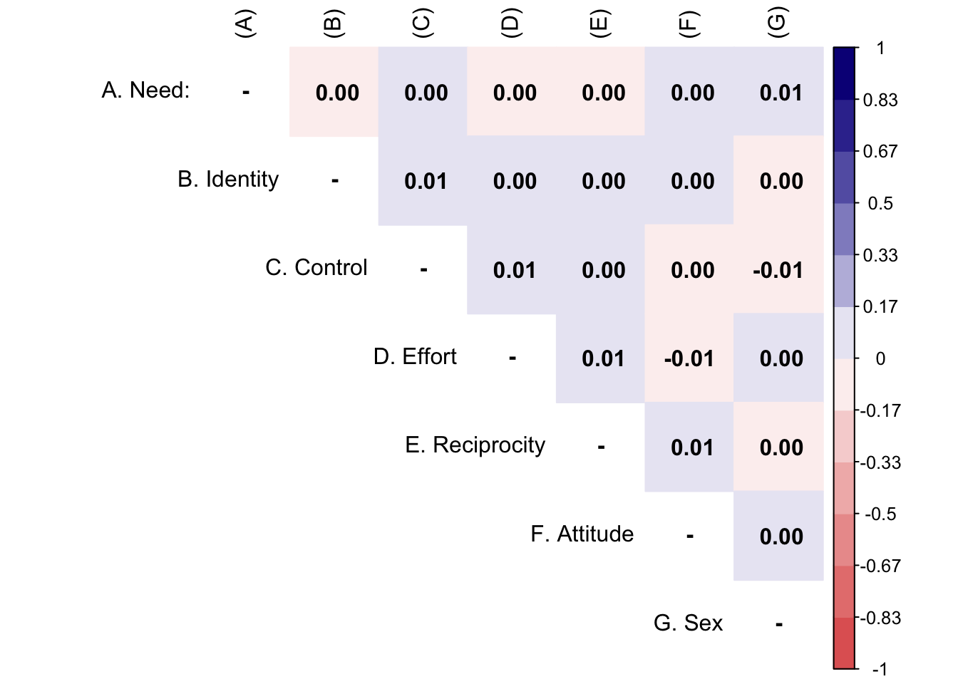
Within-profile. For each presented profile (48,000 of them: 4,000 respondents × 6 tasks × 2 alternatives). Under complete independent randomization these correlations should be indistinguishable from zero.
dummy_df<-long_df|>mutate(across(all_of(attr_cols), factor))|>select(all_of(attr_cols))#mm <- model.matrix(~ ., data = dummy_df)[, -1]mm<-dummy_df|>mutate_all(~as.numeric(.))cor_within<-cor(mm)diag(cor_within)<-NArownames(cor_within)<-c("A. Need:","B. Identity","C. Control","D. Effort","E. Reciprocity","F. Attitude","G. Sex")#set Column names of the matrixcolnames(cor_within)<-c("(A)", "(B)","(C)","(D)","(E)","(F)","(G)")testp<-cor.mtest(cor_within, conf.level =0.95)#Plot the matrix using corrplotcorrplot::corrplot(cor_within, method ="color", addCoef.col ="black", type ="upper", tl.col ="black", col =colorRampPalette(c("#E16462", "white", "#0D0887"))(12), bg ="white", na.label ="-")
With 48,000 simulated profiles, the sampling standard error of a correlation under the null of true independence is \(1/\sqrt{48,000} \approx 0.0046\), so correlations within \(\pm0.0137\) (three standard errors) are indistinguishable from sampling noise. The observed maximum, 0.0107, falls inside that band.
Robustness across sample sizes. The check above uses the full \(N = 4{,}000\) simulated sample. To confirm that the near-zero correlations are a small-sample-noise phenomenon that shrinks with \(N\) — rather than an artifact of averaging over a large sample — the same within-profile check (one numeric column per attribute, off-diagonal correlations) is repeated at \(N =\) 500, 1,000, 1,500 and 4,000 respondents, 6 tasks each. Each run reuses gen_batch() for the pairwise-restricted draws and adds sex independently per profile, exactly as in the rest of this appendix.
The 3-SE band widens as \(N\) shrinks — from $$0.0137 at \(N=4{,}000\) to $$0.0387 at \(N=500\) — and the observed maximum \(|r|\) widens along with it (0.026 at \(N=500\) down to 0.0124 at \(N=4{,}000\)), staying inside the band at every \(N\) tested. That the maximum tracks the shrinking band rather than sitting at a fixed floor is the signature of sampling noise around a true zero correlation, not of a residual structural dependence a larger sample would eventually reveal.
Between profiles, within the same task. The restriction (differ on ≥2 attributes) is a constraint on the pair, so some negative dependence between the two profiles of a task is expected and is not a threat to identification — it is orthogonal to (does not touch) the within-profile independence checked above.
Mean cross-profile correlation: -0.006 (slightly negative, as expected from the restriction). Maximum \(|r|\): 0.0545. This dependence is between the two profiles of a task, not between attributes within a profile — it plays no role in AMCE identification, which conditions on one profile’s own attribute vector (see main design chapter, Causal identification and Restrictions).
9.2.8 Summary
Under the randomization exactly as coded in app.R — independent uniform draws per attribute, with a pair redrawn only when its six CARIN/NICER attributes differ on fewer than two of them, and sex assigned independently afterward — the simulated data show: (i) near-complete coverage of the 288-profile space (288/288 profiles observed, 134–212 appearances each); (ii) uniform level balance within every attribute; (iii) within-profile attribute correlations indistinguishable from sampling noise (max \(|r|\) = 0.0107, against a 0.0137 three-SE band); and (iv) a between-profile, within-task correlation that is mildly negative, as the pairwise restriction predicts, but structurally separate from within-profile orthogonality.
9.3 Attribute-order diagnostic (mechanics only)
app.R persists the display order of the six explicit attributes per respondent as a 6-letter NICERA code (Section 9.2.4). Hainmueller et al. (2014), sec. 5.3.4, recommend testing whether an attribute’s estimated effect depends on the screen position it was shown in, via a joint Wald test on an attribute-level × position interaction. The code below implements that test end to end: parsing the NICERA code back into a per-attribute, per-respondent position, joining it to the long-format data, and running the joint interaction test.
code_to_attr<-c(N ="need", I ="identity", C ="control", E ="effort", R ="reciprocity", A ="attitude")attr_position<-function(nicera_code, attribute){map_int(str_split(nicera_code, ""), function(letters_seq){which(code_to_attr[letters_seq]==attribute)})}position_df<-purrr::map_dfc(attr_names, function(a){tibble(!!paste0("pos_", a):=attr_position(sim_db$cbc_attr_order, a))})|>mutate(session_id =sim_db$session_id, .before =1)head(position_df)
Round-trip validation (single case). Before either pipeline (reshape or NICERA decoding) is trusted on the real pilot export, both are checked end to end on one randomly chosen simulated respondent: (a) the raw cbc_profiles JSON for that respondent is parsed independently of the reshape_one() pipeline and compared, value by value, against what long_df produced for that respondent’s first task/first alternative; (b) the NICERA code stored in sim_db$cbc_attr_order is decoded with code_to_attr and compared against the original attribute-order permutation drawn for that respondent in attr_order_mat — the ground truth, which is otherwise never consulted again once the code is generated. Passing both is a necessary (not sufficient) condition for trusting the pipeline on real data: it catches encoding/decoding bugs that a check run only on the simulator’s own generative assumptions would not.
set.seed(99)check_session<-sample(sim_db$session_id, 1)# (a) Reshape: raw JSON for q1/a1 vs. what long_df producedraw_q1a1<-fromJSON(sim_db$cbc_profiles[sim_db$session_id==check_session], simplifyVector =FALSE)$q1$a1raw_q1a1_vec<-unlist(raw_q1a1)[c(attr_names, "nombre")]long_q1a1<-long_df|>filter(session_id==check_session, task==1, altID==1)|>select(all_of(attr_names), nombre)|>unlist()reshape_match<-identical(unname(raw_q1a1_vec), unname(long_q1a1))# (b) NICERA: decoded stored code vs. the original permutation drawn for this respondentoriginal_perm<-attr_order_mat[check_session, ]stored_code<-sim_db$cbc_attr_order[sim_db$session_id==check_session]recovered_perm<-unname(code_to_attr[str_split(stored_code, "")[[1]]])nicera_match<-identical(unname(original_perm), recovered_perm)roundtrip_results<-tibble( Check =c("Reshape (JSON -> long_df)", "NICERA (code -> attr_order_mat)"), Session =check_session, Detail =c(paste0("q1/a1 attributes (", paste(attr_names, collapse =", "), ", nombre)"),paste0("stored code '", stored_code, "' decoded vs. original permutation")), Pass =c(reshape_match, nicera_match))roundtrip_results|>kbl(row.names =FALSE)|>kable_styling(bootstrap_options =c("striped", "condensed"), full_width =TRUE)
Part (a) verifies that unnesting the JSON into one row per session × task × alternative did not drop, shift, or relabel any attribute along the way; part (b) verifies that the NICERA code is a lossless encoding of the display-order permutation. Checking one concrete, real case round-trip end to end catches indexing and ordering bugs that a check written against the simulator’s own assumptions (e.g. re-deriving the answer with the same logic used to produce it) would not; the stopifnot() above makes the render fail loudly rather than let either pipeline silently drift once this appendix is pointed at the real pilot export.
These results are not evidence of anything about the real instrument. The outcome fed into this test is the placeholder share generated in Section 9.2.4 — random noise, uncorrelated by construction with position or attribute level — so a null result here is guaranteed and validates only the mechanics of the parsing and testing code (NICERA decoding, position joining, interaction specification, joint Wald test), not the absence of order effects. The substantive version of this test will be run once on real pilot data, where cbc_attr_order reflects what respondents actually saw and share reflects what they actually allocated.
Hainmueller, J., Hopkins, D. J., & Yamamoto, T. (2014). Causal Inference in Conjoint Analysis: Understanding Multidimensional Choices via Stated Preference Experiments. Political Analysis, 22(1), 1–30. https://doi.org/10.1093/pan/mpt024