1 Presentation
This is the analysis code for the paper “Changes in the Justification of Pension Inequality in Chile (2016–2023) and its Relationship to Social Class and Beliefs in Meritocracy”. The dataset used is df_balanced_income.RData.
2 Libraries
3 Data
Show the code
load(file = here("input/data/rob_income/df_balanced_rob_income.RData"))

glimpse(df_balanced)
Rows: 7,968
Columns: 17
$ idencuesta <dbl> 1101011, 1101011, 1101011, 1101011, 1101011, 110…
$ ola <chr> "2016", "2017", "2018", "2019", "2022", "2023", …
$ muestra <dbl> 1, 1, 1, 1, 1, 1, 1, 1, 1, 1, 1, 1, 1, 1, 1, 1, …
$ ponderador_long_total <dbl> 0.11821742, 0.16716225, 0.15261954, 0.33262422, …
$ segmento <dbl> 110101, 110101, 110101, 110101, 110101, 110101, …
$ estrato <dbl> 4, 4, 4, 4, 4, 4, 4, 4, 4, 4, 4, 4, 4, 4, 4, 4, …
$ just_pension <fct> Strongly disagree, Strongly disagree, Strongly d…
$ merit_effort <fct> Agree, Disagree, Agree, Disagree, Disagree, Disa…
$ merit_talent <fct> Agree, Disagree, Neither agree nor disagree, Dis…
$ educ <fct> Less than Universitary, Less than Universitary, …
$ educyear <dbl> 4.30, 4.30, 7.50, 4.30, 4.30, 4.30, 9.80, 9.80, …
$ sex <fct> Female, Female, Female, Female, Female, Female, …
$ age <dbl> 64, 65, 66, 68, 70, 70, 60, 62, 62, 64, 67, 66, …
$ aget <fct> 50-64, 65 or more, 65 or more, 65 or more, 65 or…
$ ideo <fct> Does not identify, Does not identify, Right, Lef…
$ decile_eq <fct> 3, 1, 1, 1, NA, 4, 7, 8, 8, 2, NA, 1, 9, NA, NA,…
$ decile_eq1 <fct> 3, 1, 1, 1, DNA, 4, 7, 8, 8, 2, DNA, 1, 9, DNA, …Show the code
# Generate analytical sample

df_study1 <- df_balanced %>%
  select(-muestra) %>%
  na.omit() %>%
  mutate(ola = case_when(ola == "2016" ~ 1,
                         ola == "2017" ~ 2,
                         ola == "2018" ~ 3,
                         ola == "2019" ~ 4,
                         ola == "2022" ~ 5,
                         ola == "2023" ~ 6)) %>%
  mutate(ola = as.factor(ola),
         ola_num = as.numeric(ola),
         ola_2=as.numeric(ola)^2)

df_study1 <- df_study1 %>%
  group_by(idencuesta) %>%             # Agrupar por el identificador del participante
  mutate(n_participaciones = n()) %>%  # Contar el número de filas (participaciones) por participante
  ungroup()

df_study1 <- df_study1 %>% filter(n_participaciones>1)

# Corregir etiquetas

df_study1$just_pension <- sjlabelled::set_label(df_study1$just_pension,
                        label = "Pension distributive justice")

df_study1$egp <- sjlabelled::set_label(df_study1$egp,
                        label = "Social class")

df_study1$merit_effort <- sjlabelled::set_label(df_study1$merit_effort,
                        label = "People are rewarded for their efforts")

df_study1$merit_talent <- sjlabelled::set_label(df_study1$merit_talent,
                        label = "People are rewarded for their intelligence")
4 Analysis
4.1 Descriptives
Show the code
datos.pension <- df_study1 %>%
   mutate(just_pension = factor(just_pension,
                              levels = c("Strongly agree",
                                         "Agree",
                                         "Neither agree nor disagree",
                                         "Disagree",
                                         "Strongly disagree"))) %>%
  group_by(idencuesta, ola) %>%
  count(just_pension) %>%
  group_by(ola) %>%
  mutate(porcentaje=n/sum(n)) %>%
  ungroup() %>%
  na.omit() %>%
  mutate(wave = case_when(ola == 1 ~ "2016",
                          ola == 2 ~ "2017",
                          ola == 3 ~ "2018",
                          ola == 4 ~ "2019",
                          ola == 5 ~ "2022",
                          ola == 6 ~ "2023"),
         wave = factor(wave, levels = c("2016",
                                        "2017",
                                        "2018",
                                        "2019",
                                        "2022",
                                        "2023")))


etiquetas.pension <- df_study1 %>%
  mutate(just_pension = factor(just_pension,
                              levels = c("Strongly agree",
                                         "Agree",
                                         "Neither agree nor disagree",
                                         "Disagree",
                                         "Strongly disagree"))) %>%
  group_by(ola, just_pension) %>%
  summarise(count = n(), .groups = "drop") %>%
  group_by(ola) %>%
  mutate(porcentaje = count / sum(count)) %>%
  na.omit() %>%
  mutate(idencuesta = 1,
         wave = case_when(ola == 1 ~ "2016",
                          ola == 2 ~ "2017",
                          ola == 3 ~ "2018",
                          ola == 4 ~ "2019",
                          ola == 5 ~ "2022",
                          ola == 6 ~ "2023"),
         wave = factor(wave, levels = c("2016",
                                        "2017",
                                        "2018",
                                        "2019",
                                        "2022",
                                        "2023")))


datos.pension %>%
  ggplot(aes(x = wave, fill = just_pension, stratum = just_pension,
             alluvium = idencuesta, y = porcentaje)) +
  ggalluvial::geom_flow(alpha = .4) +
  ggalluvial::geom_stratum(linetype = 0) +
  scale_y_continuous(labels = scales::percent) +
  scale_fill_manual(values =  c("#0571B0","#92C5DE","#b3b3b3ff","#F4A582","#CA0020")) +
  geom_shadowtext(data = etiquetas.pension,
                  aes(label = ifelse(porcentaje > 0 , scales::percent(porcentaje, accuracy = .1),"")),
                  position = position_stack(vjust = .5),
                  show.legend = FALSE,
                  size = 3,
                  color = rep('white'),
                  bg.colour='grey30')+
  labs(y = "%",
       x = NULL,
       fill = NULL,
       title = NULL) +
  theme_ggdist() +
theme(legend.position = "bottom") 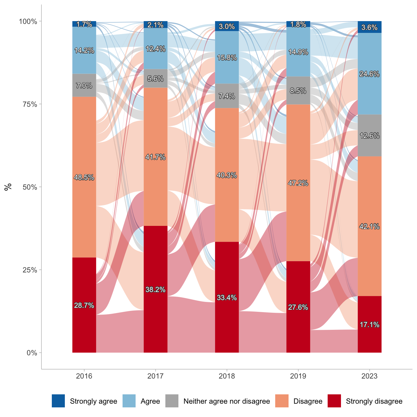
4.2 Longitudinal multilevel models
4.3 ICC
Show the code
m0 <- clmm(just_pension ~ 1 + (1 | idencuesta),
           link = "logit",
  Hess = TRUE, # calcula explícitamente la matriz varianza-covarianza de estimadores
                data = df_study1)

performance::icc(m0, by_group = T) # 0.23 es between, 0.77 within
# ICC by Group
Group | ICC
------------------
idencuesta | 0.2264.4 Time effects
Show the code
#m1.1 <- clmm(just_pension ~ 1 + ola + (1 | idencuesta),
#                link = "logit",
#  Hess = TRUE,
#  data = df_study1)
#
#m1.2 <- clmm(just_pension ~ 1 + ola_num + (1 | idencuesta),
#                link = "logit",
#  Hess = TRUE, data = df_study1)
#
#m1.3 <- clmm(just_pension ~ 1 + ola_num + ola_2 + (1| idencuesta),
#                link = "logit",
#  Hess = TRUE, data = df_study1)
#
#m1.4 <- clmm(just_pension ~ 1 + ola_num + ola_2 + (1 + ola_num | #idencuesta),
#               link = "logit",
# Hess = TRUE, data = df_study1)
#
##save(m1.1,m1.2,m1.3,m1.4, file = here("output/rob_income/time_effects.RData"))

load(file = here("output/rob_income/time_effects.RData"))

ccoef <- list(
  "Strongly disagree|Disagree" = "Strongly disagree|Disagree",
  "Disagree|Neither agree nor disagree" = "Disagree|Neither agree nor disagree",
  "Neither agree nor disagree|Agree" = "Neither agree nor disagree|Agree",
  "Agree|Strongly agree" = "Agree|Strongly agree",
  "ola2017" = "Wave 2017",
  "ola2018" = "Wave 2018",
  "ola2019" = "Wave 2019",
  "ola2022" = "Wave 2022",
  "ola2023" = "Wave 2023",
  ola_num = "Wave",
  ola_2 = "Wave^2")

texreg::htmlreg(list(m1.1,m1.2,m1.3,m1.4),
               caption.above = T,
               caption = NULL,
               stars = c(0.05, 0.01, 0.001),
               custom.coef.map = ccoef,
               digits = 3,
               groups = list("Wave (Ref.= 2016)" = 5:9),
               custom.note = "Note: Cells contain regression coefficients with standard errors in parentheses. %stars.",
               leading.zero = T,
               use.packages = F,
               booktabs = F,
               scalebox = 0.80,
               include.loglik = FALSE,
               include.aic = FALSE,
center = T)| Model 1 | Model 2 | Model 3 | Model 4 | |
|---|---|---|---|---|
| Strongly disagree|Disagree | -1.030*** | -0.498*** | -1.510*** | -1.513*** |
| (0.065) | (0.066) | (0.123) | (0.123) | |
| Disagree|Neither agree nor disagree | 1.327*** | 1.820*** | 0.842*** | 0.838*** |
| (0.066) | (0.071) | (0.122) | (0.121) | |
| Neither agree nor disagree|Agree | 1.912*** | 2.396*** | 1.425*** | 1.422*** |
| (0.070) | (0.075) | (0.123) | (0.123) | |
| Agree|Strongly agree | 4.419*** | 4.879*** | 3.927*** | 3.931*** |
| (0.109) | (0.113) | (0.148) | (0.148) | |
| Wave (Ref.= 2016) | ||||
| Wave 2017 | -0.368*** | |||
| (0.081) | ||||
| Wave 2018 | -0.024 | |||
| (0.078) | ||||
| Wave 2019 | 0.086 | |||
| (0.076) | ||||
| Wave 2023 | 0.842*** | |||
| (0.077) | ||||
| Wave | 0.209*** | -0.652*** | -0.653*** | |
| (0.017) | (0.090) | (0.090) | ||
| Wave^2 | 0.144*** | 0.144*** | ||
| (0.015) | (0.015) | |||
| BIC | 15519.842 | 15604.978 | 15517.638 | 15534.327 |
| Num. obs. | 6123 | 6123 | 6123 | 6123 |
| Groups (idencuesta) | 1327 | 1327 | 1327 | 1327 |
| Variance: idencuesta: (Intercept) | 1.064 | 1.019 | 1.056 | 0.939 |
| Variance: idencuesta: ola_num | 0.000 | |||
| Note: Cells contain regression coefficients with standard errors in parentheses. ***p < 0.001; **p < 0.01; *p < 0.05. | ||||
4.4.1 Anova
Show the code
anova(m1.3, m1.4) # quedarse con tiempo continua y con pendiente aleatoriaLikelihood ratio tests of cumulative link models:
formula: link:
m1.3 just_pension ~ 1 + ola_num + ola_2 + (1 | idencuesta) logit
m1.4 just_pension ~ 1 + ola_num + ola_2 + (1 + ola_num | idencuesta) logit
threshold:
m1.3 flexible
m1.4 flexible
no.par AIC logLik LR.stat df Pr(>Chisq)
m1.3 7 15471 -7728.3
m1.4 9 15474 -7727.9 0.7511 2 0.68694.5 WE and BE main effects
| Model 1 | Model 2 | Model 3 | Model 4 | Model 5 | Model 6 | Model 7 | |
|---|---|---|---|---|---|---|---|
| Wave 2017 | -0.368*** | ||||||
| (0.081) | |||||||
| Wave 2018 | -0.024 | ||||||
| (0.078) | |||||||
| Wave 2019 | 0.086 | ||||||
| (0.076) | |||||||
| Wave 2023 | 0.842*** | ||||||
| (0.077) | |||||||
| Wave | -0.653*** | -0.675*** | -0.678*** | -0.680*** | -0.681*** | -0.685*** | |
| (0.090) | (0.090) | (0.090) | (0.090) | (0.090) | (0.090) | ||
| Wave^2 | 0.144*** | 0.148*** | 0.148*** | 0.148*** | 0.148*** | 0.148*** | |
| (0.015) | (0.015) | (0.015) | (0.015) | (0.015) | (0.015) | ||
| Merit: Effort (WE) | 0.145*** | 0.147*** | 0.148*** | 0.148*** | 0.142*** | ||
| (0.039) | (0.039) | (0.039) | (0.039) | (0.039) | |||
| Merit: Talent (WE) | 0.071 | 0.071 | 0.070 | 0.070 | 0.066 | ||
| (0.039) | (0.039) | (0.039) | (0.039) | (0.039) | |||
| Merit: Effort (BE) | 0.333*** | 0.358*** | 0.351*** | 0.335*** | |||
| (0.090) | (0.089) | (0.088) | (0.086) | ||||
| Merit: Talent (BE) | 0.089 | 0.088 | 0.112 | 0.066 | |||
| (0.092) | (0.090) | (0.089) | (0.087) | ||||
| Decile 10 (BE) | 0.707*** | 0.537*** | 0.478*** | ||||
| (0.096) | (0.104) | (0.102) | |||||
| Universitary education (BE) | 0.385*** | 0.344*** | |||||
| (0.096) | (0.097) | ||||||
| Controls | No | No | No | No | No | No | Yes |
| BIC | 15519.842 | 15534.327 | 15510.926 | 15479.716 | 15434.695 | 15427.404 | 15399.703 |
| Numb. obs. | 6123 | 6123 | 6123 | 6123 | 6123 | 6123 | 6123 |
| Num. groups: individuals | 1327 | 1327 | 1327 | 1327 | 1327 | 1327 | 1327 |
| Var: individuals (Intercept) | 1.064 | 0.939 | 0.962 | 0.832 | 0.726 | 0.704 | 0.656 |
| Var: individuals, wave | 0.000 | 0.000 | 0.001 | 0.001 | 0.001 | 0.001 | |
| Note: Cells contain regression coefficients with standard errors in parentheses. ***p < 0.001; **p < 0.01; *p < 0.05. | |||||||
4.6 Interactions with controls (direct effect)
Show the code
 ## WE and BE Interactions with controls

#
## income
#m11 <- clmm(just_pension ~ 1 + ola_num +  ola_2 +
#               merit_effort_cwc + merit_talent_cwc +
#               merit_effort_mean + merit_talent_mean +
#               dummy_decile10_mean*merit_effort_cwc +
#               dummy_educ_mean + ideo + sex + age +
#               (1 + ola_num + merit_effort_cwc| idencuesta),
#            link = "logit",
#  Hess = TRUE,
#           data = df_study1)
#
#
#m12 <- clmm(just_pension ~ 1 + ola_num +  ola_2 +
#               merit_effort_cwc + merit_talent_cwc +
#               merit_effort_mean + merit_talent_mean +
#               dummy_decile10_mean*merit_effort_mean +
#               dummy_educ_mean + ideo + sex + age +
#               (1 + ola_num + merit_effort_mean| idencuesta),
#            link = "logit",
#  Hess = TRUE,
#           data = df_study1)
#
#m13 <- clmm(just_pension ~ 1 + ola_num +  ola_2 +
#               merit_effort_cwc + merit_talent_cwc +
#               merit_effort_mean + merit_talent_mean +
#               dummy_decile10_mean*merit_talent_cwc +
#               dummy_educ_mean + ideo + sex + age +
#               (1 + ola_num + merit_talent_cwc| idencuesta),
#            link = "logit",
#  Hess = TRUE,
#           data = df_study1)
#
#
#m14 <- clmm(just_pension ~ 1 + ola_num +  ola_2 +
#               merit_effort_cwc + merit_talent_cwc +
#               merit_effort_mean + merit_talent_mean +
#               dummy_decile10_mean*merit_talent_mean +
#               dummy_educ_mean + ideo + sex + age +
#               (1 + ola_num + merit_talent_mean| idencuesta),
#            link = "logit",
#  Hess = TRUE,
#           data = df_study1)
#
## educ
#
#
#m15 <- clmm(just_pension ~ 1 + ola_num +  ola_2 +
#              merit_effort_cwc + merit_talent_cwc +
#              merit_effort_mean + merit_talent_mean +
#              dummy_educ_mean*merit_effort_cwc +
#              dummy_decile10_mean + ideo + sex + age +
#              (1 + ola_num + merit_effort_cwc| idencuesta),
#            link = "logit",
#            Hess = TRUE,
#            data = df_study1)
#
#
#m16 <- clmm(just_pension ~ 1 + ola_num +  ola_2 +
#              merit_effort_cwc + merit_talent_cwc +
#              merit_effort_mean + merit_talent_mean +
#              dummy_educ_mean*merit_effort_mean +
#              dummy_decile10_mean + ideo + sex + age +
#              (1 + ola_num + merit_effort_mean| idencuesta),
#            link = "logit",
#            Hess = TRUE,
#            data = df_study1)
#
#m17 <- clmm(just_pension ~ 1 + ola_num +  ola_2 +
#              merit_effort_cwc + merit_talent_cwc +
#              merit_effort_mean + merit_talent_mean +
#              dummy_educ_mean*merit_talent_cwc +
#              dummy_decile10_mean + ideo + sex + age +
#              (1 + ola_num + merit_talent_cwc| idencuesta),
#            link = "logit",
#            Hess = TRUE,
#            data = df_study1)
#
#
#m18 <- clmm(just_pension ~ 1 + ola_num +  ola_2 +
#              merit_effort_cwc + merit_talent_cwc +
#              merit_effort_mean + merit_talent_mean +
#              dummy_educ_mean*merit_talent_mean +
#              dummy_decile10_mean + ideo + sex + age +
#              (1 + ola_num + merit_talent_mean| idencuesta),
#            link = "logit",
#            Hess = TRUE,
#            data = df_study1)
#
#save(m11,m12,m13,m14,m15,m16,m17,m18,file = #here("output/rob_income/interactions_direct.RData"))

load(file = here("output/rob_income/interactions_direct.RData"))

htmlreg(list(m11,m12,m13,m14))| Model 1 | Model 2 | Model 3 | Model 4 | |
|---|---|---|---|---|
| ola_num | -0.69*** | -0.69 | -0.69*** | -0.69*** |
| (0.09) | (0.09) | (0.09) | ||
| ola_2 | 0.15*** | 0.15 | 0.15*** | 0.15*** |
| (0.02) | (0.02) | (0.01) | ||
| merit_effort_cwc | 0.15*** | 0.14 | 0.15*** | 0.14*** |
| (0.04) | (0.04) | (0.04) | ||
| merit_talent_cwc | 0.06 | 0.07 | 0.08 | 0.07 |
| (0.04) | (0.04) | (0.04) | ||
| merit_effort_mean | 0.33*** | 0.27 | 0.34*** | 0.34*** |
| (0.09) | (0.09) | (0.08) | ||
| merit_talent_mean | 0.06 | 0.08 | 0.07 | 0.02 |
| (0.09) | (0.09) | (0.09) | ||
| dummy_decile10_mean | 0.49*** | -0.40 | 0.49*** | -0.22 |
| (0.10) | (0.10) | (0.44) | ||
| dummy_educ_mean | 0.35*** | 0.35 | 0.35*** | 0.37*** |
| (0.10) | (0.10) | (0.10) | ||
| ideoCenter | 0.32*** | 0.31 | 0.32*** | 0.32*** |
| (0.08) | (0.08) | (0.08) | ||
| ideoRight | 0.66*** | 0.65 | 0.67*** | 0.65*** |
| (0.10) | (0.10) | (0.10) | ||
| ideoDoes not identify | 0.23** | 0.22 | 0.24** | 0.23** |
| (0.08) | (0.08) | (0.08) | ||
| sexFemale | -0.38*** | -0.36 | -0.38*** | -0.36*** |
| (0.08) | (0.08) | (0.08) | ||
| age | -0.00 | -0.00 | -0.00 | -0.00 |
| (0.00) | (0.00) | (0.00) | ||
| merit_effort_cwc:dummy_decile10_mean | -0.03 | |||
| (0.09) | ||||
| Strongly disagree|Disagree | -0.40 | -0.53 | -0.37 | -0.50 |
| (0.25) | (0.25) | (0.26) | ||
| Disagree|Neither agree nor disagree | 2.02*** | 1.83 | 2.06*** | 1.86*** |
| (0.25) | (0.25) | (0.26) | ||
| Neither agree nor disagree|Agree | 2.62*** | 2.42 | 2.66*** | 2.45*** |
| (0.25) | (0.25) | (0.26) | ||
| Agree|Strongly agree | 5.18*** | 4.95 | 5.23*** | 4.98*** |
| (0.27) | (0.27) | (0.27) | ||
| merit_effort_mean:dummy_decile10_mean | 0.34 | |||
| merit_talent_cwc:dummy_decile10_mean | -0.07 | |||
| (0.09) | ||||
| merit_talent_mean:dummy_decile10_mean | 0.25 | |||
| (0.15) | ||||
| Log Likelihood | -7605.70 | -7606.31 | -7603.75 | -7607.18 |
| AIC | 15259.40 | 15260.62 | 15255.51 | 15262.35 |
| BIC | 15420.67 | 15421.90 | 15416.78 | 15423.63 |
| Num. obs. | 6123 | 6123 | 6123 | 6123 |
| Groups (idencuesta) | 1327 | 1327 | 1327 | 1327 |
| Variance: idencuesta: (Intercept) | 0.76 | 2.56 | 0.79 | 3.10 |
| Variance: idencuesta: ola_num | 0.01 | 0.00 | 0.01 | 0.01 |
| Variance: idencuesta: merit_effort_cwc | 0.14 | |||
| Variance: idencuesta: merit_effort_mean | 0.30 | |||
| Variance: idencuesta: merit_talent_cwc | 0.16 | |||
| Variance: idencuesta: merit_talent_mean | 0.34 | |||
| ***p < 0.001; **p < 0.01; *p < 0.05 | ||||
Show the code
htmlreg(list(m15,m16,m17,m18))| Model 1 | Model 2 | Model 3 | Model 4 | |
|---|---|---|---|---|
| ola_num | -0.69*** | -0.69*** | -0.69*** | -0.69*** |
| (0.09) | (0.09) | (0.09) | (0.09) | |
| ola_2 | 0.15*** | 0.15*** | 0.15*** | 0.15*** |
| (0.02) | (0.01) | (0.02) | (0.01) | |
| merit_effort_cwc | 0.14** | 0.14*** | 0.15*** | 0.14*** |
| (0.05) | (0.04) | (0.04) | (0.04) | |
| merit_talent_cwc | 0.06 | 0.07 | 0.06 | 0.07 |
| (0.04) | (0.04) | (0.05) | (0.04) | |
| merit_effort_mean | 0.33*** | 0.28** | 0.34*** | 0.31*** |
| (0.09) | (0.09) | (0.09) | (0.08) | |
| merit_talent_mean | 0.06 | 0.07 | 0.07 | 0.04 |
| (0.09) | (0.09) | (0.09) | (0.09) | |
| dummy_educ_mean | 0.35*** | -0.21 | 0.35*** | -0.28 |
| (0.10) | (0.38) | (0.10) | (0.41) | |
| dummy_decile10_mean | 0.49*** | 0.47*** | 0.49*** | 0.47*** |
| (0.10) | (0.10) | (0.10) | (0.10) | |
| ideoCenter | 0.32*** | 0.32*** | 0.32*** | 0.31*** |
| (0.08) | (0.08) | (0.08) | (0.08) | |
| ideoRight | 0.66*** | 0.65*** | 0.67*** | 0.65*** |
| (0.10) | (0.10) | (0.10) | (0.10) | |
| ideoDoes not identify | 0.23** | 0.22** | 0.24** | 0.22** |
| (0.08) | (0.08) | (0.08) | (0.08) | |
| sexFemale | -0.38*** | -0.36*** | -0.38*** | -0.36*** |
| (0.08) | (0.08) | (0.08) | (0.08) | |
| age | -0.00 | -0.00 | -0.00 | -0.00 |
| (0.00) | (0.00) | (0.00) | (0.00) | |
| merit_effort_cwc:dummy_educ_mean | 0.05 | |||
| (0.08) | ||||
| Strongly disagree|Disagree | -0.40 | -0.49 | -0.37 | -0.51 |
| (0.25) | (0.26) | (0.25) | (0.26) | |
| Disagree|Neither agree nor disagree | 2.02*** | 1.88*** | 2.06*** | 1.86*** |
| (0.25) | (0.26) | (0.25) | (0.26) | |
| Neither agree nor disagree|Agree | 2.62*** | 2.46*** | 2.66*** | 2.44*** |
| (0.25) | (0.26) | (0.25) | (0.26) | |
| Agree|Strongly agree | 5.18*** | 4.99*** | 5.23*** | 4.97*** |
| (0.27) | (0.27) | (0.27) | (0.28) | |
| merit_effort_mean:dummy_educ_mean | 0.22 | |||
| (0.14) | ||||
| merit_talent_cwc:dummy_educ_mean | 0.04 | |||
| (0.08) | ||||
| merit_talent_mean:dummy_educ_mean | 0.24 | |||
| (0.14) | ||||
| Log Likelihood | -7605.57 | -7607.56 | -7603.92 | -7607.22 |
| AIC | 15259.15 | 15263.12 | 15255.84 | 15262.44 |
| BIC | 15420.42 | 15424.40 | 15417.12 | 15423.71 |
| Num. obs. | 6123 | 6123 | 6123 | 6123 |
| Groups (idencuesta) | 1327 | 1327 | 1327 | 1327 |
| Variance: idencuesta: (Intercept) | 0.76 | 2.56 | 0.79 | 3.21 |
| Variance: idencuesta: ola_num | 0.01 | 0.00 | 0.01 | 0.01 |
| Variance: idencuesta: merit_effort_cwc | 0.14 | |||
| Variance: idencuesta: merit_effort_mean | 0.31 | |||
| Variance: idencuesta: merit_talent_cwc | 0.16 | |||
| Variance: idencuesta: merit_talent_mean | 0.36 | |||
| ***p < 0.001; **p < 0.01; *p < 0.05 | ||||
4.7 Interactions WE x Time
Show the code
# ## WE and BE Interactions with controls
#
#df_study1 <- df_study1 |>
#  mutate(
#    time  = ola_num - min(ola_num),
#    time2 = time^2
#  )
#
#m19 <- clmm(just_pension ~ 1 + time*merit_effort_cwc +
#              time2 + merit_talent_cwc +
#               merit_effort_mean + merit_talent_mean +
#               dummy_decile10_mean +
#               dummy_educ_mean + ideo + sex + age +
#               (1 + time + merit_effort_cwc| idencuesta),
#            link = "logit",
#  Hess = TRUE,
#           data = df_study1)
#
#m20 <- clmm(just_pension ~ 1 + time*merit_talent_cwc +
#              time2 +  merit_effort_cwc +
#               merit_effort_mean + merit_talent_mean +
#               dummy_decile10_mean +
#               dummy_educ_mean + ideo + sex + age +
#               (1 + time + merit_talent_cwc| idencuesta),
#            link = "logit",
#  Hess = TRUE,
#           data = df_study1)
#
#
#screenreg(list(m19, m20))
#
#m19_flex <- clmm(
#  just_pension ~ 1 + factor(ola_num)*merit_effort_cwc +
#    merit_talent_cwc +
#    merit_effort_mean + merit_talent_mean +
#    dummy_decile10_mean + dummy_educ_mean +
#    ideo + sex + age +
#    (1 + merit_effort_cwc | idencuesta),
#  link = "logit",
#  Hess = TRUE,
#  data = df_study1
#)
#
#m20_flex <- clmm(
#  just_pension ~ 1 + factor(ola_num)*merit_talent_cwc +
#    merit_effort_cwc +
#    merit_effort_mean + merit_talent_mean +
#    dummy_decile10_mean + dummy_educ_mean +
#    ideo + sex + age +
#    (1 + merit_talent_cwc | idencuesta),
#  link = "logit",
#  Hess = TRUE,
#  data = df_study1
#)
#
#screenreg(list(m19_flex, m20_flex))
#
#save(m19,m20, m19_flex, m20_flex, file = #here("output/rob_income/interactions_withinxtime.RData"))

load(file = here("output/rob_income/interactions_withinxtime.RData"))

htmlreg(list(m19, m20, m19_flex, m20_flex))| Model 1 | Model 2 | Model 3 | Model 4 | |
|---|---|---|---|---|
| time | -0.39*** | -0.39*** | ||
| (0.06) | (0.06) | |||
| merit_effort_cwc | 0.15* | 0.15*** | 0.28*** | 0.15*** |
| (0.06) | (0.04) | (0.08) | (0.04) | |
| time2 | 0.15*** | 0.15*** | ||
| (0.02) | (0.02) | |||
| merit_talent_cwc | 0.06 | 0.07 | 0.06 | 0.16* |
| (0.04) | (0.06) | (0.04) | (0.08) | |
| merit_effort_mean | 0.33*** | 0.34*** | 0.33*** | 0.34*** |
| (0.09) | (0.09) | (0.09) | (0.09) | |
| merit_talent_mean | 0.06 | 0.07 | 0.06 | 0.07 |
| (0.09) | (0.09) | (0.09) | (0.09) | |
| dummy_decile10_mean | 0.49*** | 0.49*** | 0.48*** | 0.49*** |
| (0.10) | (0.10) | (0.10) | (0.10) | |
| dummy_educ_mean | 0.35*** | 0.35*** | 0.35*** | 0.35*** |
| (0.10) | (0.10) | (0.10) | (0.10) | |
| ideoCenter | 0.32*** | 0.32*** | 0.31*** | 0.32*** |
| (0.08) | (0.08) | (0.08) | (0.08) | |
| ideoRight | 0.66*** | 0.67*** | 0.66*** | 0.67*** |
| (0.10) | (0.10) | (0.10) | (0.10) | |
| ideoDoes not identify | 0.23** | 0.24** | 0.24** | 0.25** |
| (0.08) | (0.08) | (0.08) | (0.08) | |
| sexFemale | -0.38*** | -0.38*** | -0.38*** | -0.38*** |
| (0.08) | (0.08) | (0.08) | (0.08) | |
| age | -0.00 | -0.00 | -0.00 | -0.00 |
| (0.00) | (0.00) | (0.00) | (0.00) | |
| time:merit_effort_cwc | -0.00 | |||
| (0.02) | ||||
| Strongly disagree|Disagree | 0.13 | 0.16 | 0.09 | 0.11 |
| (0.22) | (0.22) | (0.22) | (0.22) | |
| Disagree|Neither agree nor disagree | 2.55*** | 2.60*** | 2.51*** | 2.54*** |
| (0.23) | (0.23) | (0.23) | (0.23) | |
| Neither agree nor disagree|Agree | 3.15*** | 3.20*** | 3.11*** | 3.14*** |
| (0.23) | (0.23) | (0.23) | (0.23) | |
| Agree|Strongly agree | 5.71*** | 5.77*** | 5.66*** | 5.70*** |
| (0.25) | (0.25) | (0.25) | (0.25) | |
| time:merit_talent_cwc | -0.00 | |||
| (0.02) | ||||
| factor(ola_num)2 | -0.38*** | -0.39*** | ||
| (0.08) | (0.08) | |||
| factor(ola_num)3 | -0.05 | -0.05 | ||
| (0.08) | (0.08) | |||
| factor(ola_num)4 | 0.09 | 0.09 | ||
| (0.08) | (0.08) | |||
| factor(ola_num)5 | 0.84*** | 0.85*** | ||
| (0.08) | (0.08) | |||
| factor(ola_num)2:merit_effort_cwc | -0.24* | |||
| (0.11) | ||||
| factor(ola_num)3:merit_effort_cwc | -0.26* | |||
| (0.11) | ||||
| factor(ola_num)4:merit_effort_cwc | -0.11 | |||
| (0.11) | ||||
| factor(ola_num)5:merit_effort_cwc | -0.08 | |||
| (0.11) | ||||
| factor(ola_num)2:merit_talent_cwc | -0.21 | |||
| (0.11) | ||||
| factor(ola_num)3:merit_talent_cwc | -0.17 | |||
| (0.11) | ||||
| factor(ola_num)4:merit_talent_cwc | -0.07 | |||
| (0.10) | ||||
| factor(ola_num)5:merit_talent_cwc | -0.08 | |||
| (0.10) | ||||
| Log Likelihood | -7605.74 | -7604.04 | -7597.43 | -7597.95 |
| AIC | 15259.47 | 15256.09 | 15246.86 | 15247.90 |
| BIC | 15420.75 | 15417.36 | 15421.57 | 15422.61 |
| Num. obs. | 6123 | 6123 | 6123 | 6123 |
| Groups (idencuesta) | 1327 | 1327 | 1327 | 1327 |
| Variance: idencuesta: (Intercept) | 0.79 | 0.80 | 0.87 | 0.88 |
| Variance: idencuesta: time | 0.01 | 0.01 | ||
| Variance: idencuesta: merit_effort_cwc | 0.14 | 0.13 | ||
| Variance: idencuesta: merit_talent_cwc | 0.16 | 0.16 | ||
| ***p < 0.001; **p < 0.01; *p < 0.05 | ||||