1 Presentation
This is the data preparation code for the paper “Market justice preferences for education”. The prepared dataset correspond to the 1999, 2009 and 2019 Social Inequality Module of International Social Survey Programme (ISSP).
2 Libraries
3 Data
issp99 <- read_dta(here("input/data/original/issp_1999.dta"))
issp09 <- read_dta(here("input/data/original/issp_2009.dta"))
issp19 <- read_dta(here("input/data/original/issp_2019.dta"))
4 Processing ISSP 1999
4.1 Select
db_proc99 <- issp99 %>%
  select(year = v1,
         v3,
         sex,
         age,
         marital,
         educyrs,
         degree,
         rincome,
         rincomer,
         ess = v46,
         nmerit_wealthy_fam = v4,
         nmerit_contacts = v5,
         merit_effort = v6,
         merit_talent = v7,
         just_educ = v40,
         weight) %>%
  janitor::clean_names()
4.2 Recode and transform
4.2.1 Year
frq(db_proc99$year)ZA study number .... (x) <numeric>
# total N=32178 valid N=32178 mean=1999.00 sd=0.00
Value | Label | N | Raw % | Valid % | Cum. %
-------------------------------------------------
1999 | ISSP99 | 32178 | 100 | 100 | 100
<NA> | <NA> | 0 | 0 | <NA> | <NA>db_proc99$year <- as.numeric(db_proc99$year)
frq(db_proc99$year)x <numeric>
# total N=32178 valid N=32178 mean=1999.00 sd=0.00
Value | N | Raw % | Valid % | Cum. %
----------------------------------------
1999 | 32178 | 100 | 100 | 100
<NA> | 0 | 0 | <NA> | <NA>4.2.2 Country
frq(db_proc99$v3)Country (x) <numeric>
# total N=32178 valid N=32178 mean=17.13 sd=9.19
Value | Label | N | Raw % | Valid % | Cum. %
------------------------------------------------------------
1 | AUS Australia | 1672 | 5.20 | 5.20 | 5.20
2 | D-W Germany West | 921 | 2.86 | 2.86 | 8.06
3 | D-E Germany East | 511 | 1.59 | 1.59 | 9.65
4 | GB Great Britain | 804 | 2.50 | 2.50 | 12.14
5 | NIRL North Ireland | 830 | 2.58 | 2.58 | 14.72
6 | USA United States | 1272 | 3.95 | 3.95 | 18.68
7 | A Austria | 1016 | 3.16 | 3.16 | 21.83
8 | H Hungary | 1208 | 3.75 | 3.75 | 25.59
10 | IRL Ireland | 0 | 0.00 | 0.00 | 25.59
12 | N Norway | 1268 | 3.94 | 3.94 | 29.53
13 | S Sweden | 1150 | 3.57 | 3.57 | 33.10
14 | CZ Czech Rep | 1834 | 5.70 | 5.70 | 38.80
15 | SLO Slovenia | 1006 | 3.13 | 3.13 | 41.93
16 | PL Poland | 1135 | 3.53 | 3.53 | 45.46
17 | BG Bulgaria | 1102 | 3.42 | 3.42 | 48.88
18 | RUS Russia | 1705 | 5.30 | 5.30 | 54.18
19 | NZ New Zealand | 1108 | 3.44 | 3.44 | 57.62
20 | CDN Canada | 974 | 3.03 | 3.03 | 60.65
21 | RP Philippines | 1200 | 3.73 | 3.73 | 64.38
22 | IL Israel | 1208 | 3.75 | 3.75 | 68.13
24 | J Japan | 1325 | 4.12 | 4.12 | 72.25
25 | E Spain | 1211 | 3.76 | 3.76 | 76.01
26 | LV Latvia | 1100 | 3.42 | 3.42 | 79.43
27 | F France | 1889 | 5.87 | 5.87 | 85.30
28 | CY Cyprus | 1000 | 3.11 | 3.11 | 88.41
29 | P Portugal | 1144 | 3.56 | 3.56 | 91.97
30 | RCH Chile | 1503 | 4.67 | 4.67 | 96.64
33 | SVK Slovakia | 1082 | 3.36 | 3.36 | 100.00
<NA> | <NA> | 0 | 0.00 | <NA> | <NA>db_proc99 <- db_proc99 %>%
mutate(country = case_when(
v3 == 1 ~ "Australia",
v3 == 2 | v3 == 3 ~ "Germany",
v3 == 4 ~ "United Kingdom",
v3 == 5 ~ "Ireland",
v3 == 6 ~ "United States",
v3 == 7 ~ "Austria",
v3 == 8 ~ "Hungary",
v3 == 10 ~ "Ireland",
v3 == 12 ~ "Norway",
v3 == 13 ~ "Sweden",
v3 == 14 ~ "Czech Republic",
v3 == 15 ~ "Slovenia",
v3 == 16 ~ "Poland",
v3 == 17 ~ "Bulgaria",
v3 == 18 ~ "Russia",
v3 == 19 ~ "New Zealand",
v3 == 20 ~ "Canada",
v3 == 21 ~ "Philippines",
v3 == 22 ~ "Israel",
v3 == 24 ~ "Japan",
v3 == 25 ~ "Spain",
v3 == 26 ~ "Latvia",
v3 == 27 ~ "France",
v3 == 28 ~ "Cyprus",
v3 == 29 ~ "Portugal",
v3 == 30 ~ "Chile",
v3 == 33 ~ "Slovakia",
TRUE ~ NA_character_
))
db_proc99$iso_country <- countrycode::countrycode(db_proc99$country, origin = "country.name", destination = "iso3c")
frq(db_proc99$country); frq(db_proc99$iso_country)x <character>
# total N=32178 valid N=32178 mean=13.07 sd=7.44
Value | N | Raw % | Valid % | Cum. %
------------------------------------------------
Australia | 1672 | 5.20 | 5.20 | 5.20
Austria | 1016 | 3.16 | 3.16 | 8.35
Bulgaria | 1102 | 3.42 | 3.42 | 11.78
Canada | 974 | 3.03 | 3.03 | 14.81
Chile | 1503 | 4.67 | 4.67 | 19.48
Cyprus | 1000 | 3.11 | 3.11 | 22.58
Czech Republic | 1834 | 5.70 | 5.70 | 28.28
France | 1889 | 5.87 | 5.87 | 34.15
Germany | 1432 | 4.45 | 4.45 | 38.60
Hungary | 1208 | 3.75 | 3.75 | 42.36
Ireland | 830 | 2.58 | 2.58 | 44.94
Israel | 1208 | 3.75 | 3.75 | 48.69
Japan | 1325 | 4.12 | 4.12 | 52.81
Latvia | 1100 | 3.42 | 3.42 | 56.23
New Zealand | 1108 | 3.44 | 3.44 | 59.67
Norway | 1268 | 3.94 | 3.94 | 63.61
Philippines | 1200 | 3.73 | 3.73 | 67.34
Poland | 1135 | 3.53 | 3.53 | 70.87
Portugal | 1144 | 3.56 | 3.56 | 74.42
Russia | 1705 | 5.30 | 5.30 | 79.72
Slovakia | 1082 | 3.36 | 3.36 | 83.08
Slovenia | 1006 | 3.13 | 3.13 | 86.21
Spain | 1211 | 3.76 | 3.76 | 89.97
Sweden | 1150 | 3.57 | 3.57 | 93.55
United Kingdom | 804 | 2.50 | 2.50 | 96.05
United States | 1272 | 3.95 | 3.95 | 100.00
<NA> | 0 | 0.00 | <NA> | <NA>x <character>
# total N=32178 valid N=32178 mean=13.25 sd=7.53
Value | N | Raw % | Valid % | Cum. %
---------------------------------------
AUS | 1672 | 5.20 | 5.20 | 5.20
AUT | 1016 | 3.16 | 3.16 | 8.35
BGR | 1102 | 3.42 | 3.42 | 11.78
CAN | 974 | 3.03 | 3.03 | 14.81
CHL | 1503 | 4.67 | 4.67 | 19.48
CYP | 1000 | 3.11 | 3.11 | 22.58
CZE | 1834 | 5.70 | 5.70 | 28.28
DEU | 1432 | 4.45 | 4.45 | 32.73
ESP | 1211 | 3.76 | 3.76 | 36.50
FRA | 1889 | 5.87 | 5.87 | 42.37
GBR | 804 | 2.50 | 2.50 | 44.87
HUN | 1208 | 3.75 | 3.75 | 48.62
IRL | 830 | 2.58 | 2.58 | 51.20
ISR | 1208 | 3.75 | 3.75 | 54.95
JPN | 1325 | 4.12 | 4.12 | 59.07
LVA | 1100 | 3.42 | 3.42 | 62.49
NOR | 1268 | 3.94 | 3.94 | 66.43
NZL | 1108 | 3.44 | 3.44 | 69.87
PHL | 1200 | 3.73 | 3.73 | 73.60
POL | 1135 | 3.53 | 3.53 | 77.13
PRT | 1144 | 3.56 | 3.56 | 80.69
RUS | 1705 | 5.30 | 5.30 | 85.98
SVK | 1082 | 3.36 | 3.36 | 89.35
SVN | 1006 | 3.13 | 3.13 | 92.47
SWE | 1150 | 3.57 | 3.57 | 96.05
USA | 1272 | 3.95 | 3.95 | 100.00
<NA> | 0 | 0.00 | <NA> | <NA>4.2.3 Sex
frq(db_proc99$sex)R: sex (x) <numeric>
# total N=32178 valid N=32110 mean=1.52 sd=0.50
Value | Label | N | Raw % | Valid % | Cum. %
------------------------------------------------------
1 | Male | 15301 | 47.55 | 47.65 | 47.65
2 | Female | 16809 | 52.24 | 52.35 | 100.00
9 | NA, refused | 0 | 0.00 | 0.00 | 100.00
<NA> | <NA> | 68 | 0.21 | <NA> | <NA>db_proc99$sex <- set_na(db_proc99$sex, na = c(9), drop.levels = F)
db_proc99 <- db_proc99 %>%
mutate(sex = if_else(sex == 1, 'Male', 'Female'),
sex = factor(sex, levels = c("Male", "Female")))
frq(db_proc99$sex)x <categorical>
# total N=32178 valid N=32110 mean=1.52 sd=0.50
Value | N | Raw % | Valid % | Cum. %
-----------------------------------------
Male | 15301 | 47.55 | 47.65 | 47.65
Female | 16809 | 52.24 | 52.35 | 100.00
<NA> | 68 | 0.21 | <NA> | <NA>4.2.4 Age
summary(db_proc99$age) Min. 1st Qu. Median Mean 3rd Qu. Max. NA's
16.00 32.00 44.00 45.65 59.00 98.00 124 db_proc99$age <- set_na(db_proc99$age, na = c(98,99), drop.levels = F)
db_proc99$age <- as.numeric(db_proc99$age)4.2.5 Marital status
frq(db_proc99$marital)R: Marital status (x) <numeric>
# total N=32178 valid N=32012 mean=2.15 sd=1.64
Value | Label | N | Raw % | Valid % | Cum. %
--------------------------------------------------------------
1 | marr,liv as mar | 19494 | 60.58 | 60.90 | 60.90
2 | widowed | 2910 | 9.04 | 9.09 | 69.99
3 | divorced | 1980 | 6.15 | 6.19 | 76.17
4 | separated | 728 | 2.26 | 2.27 | 78.45
5 | single, not married | 6900 | 21.44 | 21.55 | 100.00
9 | NA, refused | 0 | 0.00 | 0.00 | 100.00
<NA> | <NA> | 166 | 0.52 | <NA> | <NA>db_proc99$marital <- set_na(db_proc99$marital, na = c(9), drop.levels = F)
db_proc99 <- db_proc99 %>%
mutate(marital = if_else(marital == 1, "Married", "Not married"),
marital = factor(marital, levels = c("Married", "Not married"))
)
frq(db_proc99$marital)x <categorical>
# total N=32178 valid N=32012 mean=1.39 sd=0.49
Value | N | Raw % | Valid % | Cum. %
----------------------------------------------
Married | 19494 | 60.58 | 60.90 | 60.90
Not married | 12518 | 38.90 | 39.10 | 100.00
<NA> | 166 | 0.52 | <NA> | <NA>4.2.6 Education
# Eucation
frq(db_proc99$educyrs) # We don't know if this is equal in every country; we use degree
R: Education I: years in school (x) <numeric>
# total N=32178 valid N=30327 mean=14.89 sd=15.78
Value | Label | N | Raw % | Valid % | Cum. %
-----------------------------------------------------------
0 | NAV, NAP | 0 | 0.00 | 0.00 | 0.00
1 | 1 year | 71 | 0.22 | 0.23 | 0.23
2 | 2 | 134 | 0.42 | 0.44 | 0.68
3 | 3 | 247 | 0.77 | 0.81 | 1.49
4 | 4 | 607 | 1.89 | 2.00 | 3.49
5 | 5 | 340 | 1.06 | 1.12 | 4.61
6 | 6 | 911 | 2.83 | 3.00 | 7.62
7 | 7 | 873 | 2.71 | 2.88 | 10.50
8 | 8 | 2800 | 8.70 | 9.23 | 19.73
9 | 9 | 1533 | 4.76 | 5.05 | 24.78
10 | 10 | 2167 | 6.73 | 7.15 | 31.93
11 | 11 | 3765 | 11.70 | 12.41 | 44.34
12 | 12 | 4833 | 15.02 | 15.94 | 60.28
13 | 13 | 2213 | 6.88 | 7.30 | 67.58
14 | 14 | 1733 | 5.39 | 5.71 | 73.29
15 | 15 | 1482 | 4.61 | 4.89 | 78.18
16 | 16 | 1719 | 5.34 | 5.67 | 83.85
17 | 17 | 951 | 2.96 | 3.14 | 86.98
18 | 18 | 1197 | 3.72 | 3.95 | 90.93
19 | 19 | 333 | 1.03 | 1.10 | 92.03
20 | 20 | 446 | 1.39 | 1.47 | 93.50
21 | 21 | 182 | 0.57 | 0.60 | 94.10
22 | 22 | 166 | 0.52 | 0.55 | 94.65
23 | 23 | 134 | 0.42 | 0.44 | 95.09
24 | 24 | 135 | 0.42 | 0.45 | 95.53
25 | 25 | 111 | 0.34 | 0.37 | 95.90
26 | 26 | 56 | 0.17 | 0.18 | 96.08
27 | 27 | 43 | 0.13 | 0.14 | 96.22
28 | 28 | 26 | 0.08 | 0.09 | 96.31
29 | 29 | 9 | 0.03 | 0.03 | 96.34
30 | 30 | 16 | 0.05 | 0.05 | 96.39
31 | 31 | 5 | 0.02 | 0.02 | 96.41
32 | 32 | 7 | 0.02 | 0.02 | 96.43
33 | 33 | 2 | 0.01 | 0.01 | 96.44
34 | 34 | 5 | 0.02 | 0.02 | 96.46
35 | 35 | 8 | 0.02 | 0.03 | 96.48
36 | 36 | 4 | 0.01 | 0.01 | 96.49
37 | 37 | 4 | 0.01 | 0.01 | 96.51
38 | 38 | 5 | 0.02 | 0.02 | 96.52
39 | 39 | 1 | 0.00 | 0.00 | 96.53
40 | 40 | 10 | 0.03 | 0.03 | 96.56
41 | 41 | 1 | 0.00 | 0.00 | 96.56
42 | 42 | 3 | 0.01 | 0.01 | 96.57
43 | 43 | 1 | 0.00 | 0.00 | 96.58
45 | 45 | 1 | 0.00 | 0.00 | 96.58
46 | 46 | 1 | 0.00 | 0.00 | 96.58
47 | 47 | 1 | 0.00 | 0.00 | 96.59
49 | 49 | 1 | 0.00 | 0.00 | 96.59
50 | 50 | 2 | 0.01 | 0.01 | 96.60
55 | 55 | 1 | 0.00 | 0.00 | 96.60
67 | 67 years | 1 | 0.00 | 0.00 | 96.60
93 | Other answer | 5 | 0.02 | 0.02 | 96.62
94 | Only compulsory | 0 | 0.00 | 0.00 | 96.62
95 | Still school | 326 | 1.01 | 1.07 | 97.70
96 | Still college,uni | 433 | 1.35 | 1.43 | 99.12
97 | No form school | 266 | 0.83 | 0.88 | 100.00
98 | Dont know | 0 | 0.00 | 0.00 | 100.00
99 | na | 0 | 0.00 | 0.00 | 100.00
<NA> | <NA> | 1851 | 5.75 | <NA> | <NA>frq(db_proc99$degree)R: Education II: categories (x) <numeric>
# total N=32178 valid N=30939 mean=4.65 sd=1.47
Value | Label | N | Raw % | Valid % | Cum. %
----------------------------------------------------------
1 | None | 442 | 1.37 | 1.43 | 1.43
2 | Incpl primary | 1530 | 4.75 | 4.95 | 6.37
3 | Primary compl | 4957 | 15.40 | 16.02 | 22.40
4 | Incpl secondary | 7640 | 23.74 | 24.69 | 47.09
5 | Secondary compl | 8124 | 25.25 | 26.26 | 73.35
6 | Incpl university | 3435 | 10.67 | 11.10 | 84.45
7 | University compl | 4811 | 14.95 | 15.55 | 100.00
8 | Cant choose | 0 | 0.00 | 0.00 | 100.00
9 | na | 0 | 0.00 | 0.00 | 100.00
<NA> | <NA> | 1239 | 3.85 | <NA> | <NA>db_proc99$degree <- set_na(db_proc99$degree, na = c(8,9), drop.levels = F)
db_proc99 <- db_proc99 %>%
mutate(educ = case_when(degree %in% c(1,2) ~ "Incomplete primary or less",
degree == 3 ~ "Complete primary",
degree == 4 ~ "Incomplete secondary",
degree == 5 ~ "Complete secondary",
degree == 6 ~ "Incomplete university",
degree == 7 ~ "Complete university",
TRUE ~ NA_character_),
educ = factor(educ,
levels = c("Incomplete primary or less",
"Complete primary",
"Incomplete secondary",
"Complete secondary",
"Incomplete university",
"Complete university")))
db_proc99 <- db_proc99 %>%
mutate(educ_dic = case_when(degree %in% c(1:6) ~ 'Less than universitary',
degree == 7 ~ 'Universitary',
TRUE ~ NA_character_),
educ_dic = factor(educ_dic, levels = c("Universitary", "Less than universitary")))
frq(db_proc99$educ)x <categorical>
# total N=32178 valid N=30939 mean=3.66 sd=1.44
Value | N | Raw % | Valid % | Cum. %
------------------------------------------------------------
Incomplete primary or less | 1972 | 6.13 | 6.37 | 6.37
Complete primary | 4957 | 15.40 | 16.02 | 22.40
Incomplete secondary | 7640 | 23.74 | 24.69 | 47.09
Complete secondary | 8124 | 25.25 | 26.26 | 73.35
Incomplete university | 3435 | 10.67 | 11.10 | 84.45
Complete university | 4811 | 14.95 | 15.55 | 100.00
<NA> | 1239 | 3.85 | <NA> | <NA>frq(db_proc99$educ_dic)x <categorical>
# total N=32178 valid N=30939 mean=1.84 sd=0.36
Value | N | Raw % | Valid % | Cum. %
---------------------------------------------------------
Universitary | 4811 | 14.95 | 15.55 | 15.55
Less than universitary | 26128 | 81.20 | 84.45 | 100.00
<NA> | 1239 | 3.85 | <NA> | <NA>4.2.7 Income
# Income continuous
summary(db_proc99$rincome)
Min. 1st Qu. Median Mean 3rd Qu. Max. NA's
0 3 500 109418 13250 999999 79 db_proc99 <- db_proc99 %>%
mutate(
rincome = haven::zap_labels(rincome),
rincome = sjmisc::set_na(rincome, na = c(999997,999998,999999))
)
# ntile function without NAs
ntile_na <- function(x,n)
{
notna <- !is.na(x)
out <- rep(NA_real_,length(x))
out[notna] <- ntile(x[notna],n)
return(out)
}
db_proc99 %>%
mutate(decil = ntile_na(rincome, 10)) %>%
frq(decil)decil <numeric>
# total N=32178 valid N=28811 mean=5.50 sd=2.87
Value | N | Raw % | Valid % | Cum. %
---------------------------------------
1 | 2882 | 8.96 | 10 | 10
2 | 2881 | 8.95 | 10 | 20
3 | 2881 | 8.95 | 10 | 30
4 | 2881 | 8.95 | 10 | 40
5 | 2881 | 8.95 | 10 | 50
6 | 2881 | 8.95 | 10 | 60
7 | 2881 | 8.95 | 10 | 70
8 | 2881 | 8.95 | 10 | 80
9 | 2881 | 8.95 | 10 | 90
10 | 2881 | 8.95 | 10 | 100
<NA> | 3367 | 10.46 | <NA> | <NA># Income decil
frq(db_proc99$rincomer) R: Earnings II: categories (x) <numeric>
# total N=32178 valid N=32154 mean=12.07 sd=27.95
Value | Label | N | Raw % | Valid % | Cum. %
-------------------------------------------------------------------------
0 | Nap, n force laboral, no income | 5995 | 18.63 | 18.64 | 18.64
1 | Lowest decile | 3556 | 11.05 | 11.06 | 29.70
2 | 2 | 4412 | 13.71 | 13.72 | 43.43
3 | 3 | 3304 | 10.27 | 10.28 | 53.70
4 | 4 | 3508 | 10.90 | 10.91 | 64.61
5 | 5 | 3122 | 9.70 | 9.71 | 74.32
6 | 6 | 2126 | 6.61 | 6.61 | 80.93
7 | 7 | 1217 | 3.78 | 3.78 | 84.72
8 | 8 | 779 | 2.42 | 2.42 | 87.14
9 | 9 | 550 | 1.71 | 1.71 | 88.85
10 | Highest decile | 557 | 1.73 | 1.73 | 90.58
97 | Refused | 651 | 2.02 | 2.02 | 92.61
98 | Don't know | 437 | 1.36 | 1.36 | 93.97
99 | No answer | 1940 | 6.03 | 6.03 | 100.00
<NA> | <NA> | 24 | 0.07 | <NA> | <NA>db_proc99$rincomer <- set_na(db_proc99$rincomer, na = c(97,98,99), drop.levels = F) # there is a decil 0; those no income no labor force
db_proc99$income_decil <- as.numeric(db_proc99$rincomer)
frq(db_proc99$income_decil) x <numeric>
# total N=32178 valid N=29126 mean=3.09 sd=2.58
Value | N | Raw % | Valid % | Cum. %
---------------------------------------
0 | 5995 | 18.63 | 20.58 | 20.58
1 | 3556 | 11.05 | 12.21 | 32.79
2 | 4412 | 13.71 | 15.15 | 47.94
3 | 3304 | 10.27 | 11.34 | 59.28
4 | 3508 | 10.90 | 12.04 | 71.33
5 | 3122 | 9.70 | 10.72 | 82.05
6 | 2126 | 6.61 | 7.30 | 89.35
7 | 1217 | 3.78 | 4.18 | 93.52
8 | 779 | 2.42 | 2.67 | 96.20
9 | 550 | 1.71 | 1.89 | 98.09
10 | 557 | 1.73 | 1.91 | 100.00
<NA> | 3052 | 9.48 | <NA> | <NA>4.2.9 Meritocratic variables
frq(db_proc99$merit_effort)People get rewarded for their effort (x) <numeric>
# total N=32178 valid N=32178 mean=3.39 sd=1.44
Value | Label | N | Raw % | Valid % | Cum. %
--------------------------------------------------------------------
1 | Strongly agree | 1596 | 4.96 | 4.96 | 4.96
2 | Agree | 8660 | 26.91 | 26.91 | 31.87
3 | Neither agree nor disagree | 6883 | 21.39 | 21.39 | 53.26
4 | Disagree | 8985 | 27.92 | 27.92 | 81.19
5 | Strongly disagree | 5034 | 15.64 | 15.64 | 96.83
8 | Cant choose | 811 | 2.52 | 2.52 | 99.35
9 | No answer | 209 | 0.65 | 0.65 | 100.00
<NA> | <NA> | 0 | 0.00 | <NA> | <NA>frq(db_proc99$merit_talent)People get rewarded for their skills (x) <numeric>
# total N=32178 valid N=32178 mean=3.22 sd=1.50
Value | Label | N | Raw % | Valid % | Cum. %
---------------------------------------------------------------------
1 | Strongly agree | 1818 | 5.65 | 5.65 | 5.65
2 | Agree | 10785 | 33.52 | 33.52 | 39.17
3 | Neither agree nor disagree | 6954 | 21.61 | 21.61 | 60.78
4 | Disagree | 7632 | 23.72 | 23.72 | 84.50
5 | Strongly disagree | 3784 | 11.76 | 11.76 | 96.26
8 | Cant choose | 941 | 2.92 | 2.92 | 99.18
9 | No answer | 264 | 0.82 | 0.82 | 100.00
<NA> | <NA> | 0 | 0.00 | <NA> | <NA>db_proc99 <- db_proc99 %>%
mutate(
across(
.cols = c(merit_effort, merit_talent),
.fns = ~ set_na(., na = c(8,9), drop.levels = F)
)
) # ok
db_proc99$merit_effort <- sjmisc::rec(db_proc99$merit_effort,rec = "rev")
db_proc99$merit_talent <- sjmisc::rec(db_proc99$merit_talent,rec = "rev")
frq(db_proc99$merit_effort)People get rewarded for their effort (x) <numeric>
# total N=32178 valid N=31158 mean=2.77 sd=1.17
Value | Label | N | Raw % | Valid % | Cum. %
--------------------------------------------------------------------
1 | Strongly disagree | 5034 | 15.64 | 16.16 | 16.16
2 | Disagree | 8985 | 27.92 | 28.84 | 44.99
3 | Neither agree nor disagree | 6883 | 21.39 | 22.09 | 67.08
4 | Agree | 8660 | 26.91 | 27.79 | 94.88
5 | Strongly agree | 1596 | 4.96 | 5.12 | 100.00
<NA> | <NA> | 1020 | 3.17 | <NA> | <NA>frq(db_proc99$merit_talent)People get rewarded for their skills (x) <numeric>
# total N=32178 valid N=30973 mean=2.97 sd=1.15
Value | Label | N | Raw % | Valid % | Cum. %
---------------------------------------------------------------------
1 | Strongly disagree | 3784 | 11.76 | 12.22 | 12.22
2 | Disagree | 7632 | 23.72 | 24.64 | 36.86
3 | Neither agree nor disagree | 6954 | 21.61 | 22.45 | 59.31
4 | Agree | 10785 | 33.52 | 34.82 | 94.13
5 | Strongly agree | 1818 | 5.65 | 5.87 | 100.00
<NA> | <NA> | 1205 | 3.74 | <NA> | <NA>4.2.10 Non-meritocratic variables
frq(db_proc99$nmerit_wealthy_fam)Importance: coming from a wealthy famil (x) <numeric>
# total N=32178 valid N=32178 mean=3.19 sd=1.41
Value | Label | N | Raw % | Valid % | Cum. %
--------------------------------------------------------------
1 | Essential | 3152 | 9.80 | 9.80 | 9.80
2 | Very important | 7004 | 21.77 | 21.77 | 31.56
3 | Fairly important | 9780 | 30.39 | 30.39 | 61.96
4 | Not very important | 7899 | 24.55 | 24.55 | 86.50
5 | Not important at all | 3493 | 10.86 | 10.86 | 97.36
8 | Cant choose | 633 | 1.97 | 1.97 | 99.33
9 | No answer | 217 | 0.67 | 0.67 | 100.00
<NA> | <NA> | 0 | 0.00 | <NA> | <NA>frq(db_proc99$nmerit_contacts)Importance: Knowing the right people (x) <numeric>
# total N=32178 valid N=32178 mean=2.59 sd=1.33
Value | Label | N | Raw % | Valid % | Cum. %
---------------------------------------------------------------
1 | Essential | 5521 | 17.16 | 17.16 | 17.16
2 | Very important | 11486 | 35.70 | 35.70 | 52.85
3 | Fairly important | 10064 | 31.28 | 31.28 | 84.13
4 | Not very important | 3307 | 10.28 | 10.28 | 94.41
5 | Not important at all | 1052 | 3.27 | 3.27 | 97.68
8 | Cant choose | 518 | 1.61 | 1.61 | 99.29
9 | No answer | 230 | 0.71 | 0.71 | 100.00
<NA> | <NA> | 0 | 0.00 | <NA> | <NA>db_proc99 <- db_proc99 %>%
mutate(
across(
.cols = c(nmerit_wealthy_fam, nmerit_contacts),
.fns = ~ set_na(., na = c(8,9), drop.levels = F)
)
) # ok
db_proc99$nmerit_wealthy_fam <- sjmisc::rec(db_proc99$nmerit_wealthy_fam,rec = "rev")
db_proc99$nmerit_contacts <- sjmisc::rec(db_proc99$nmerit_contacts,rec = "rev")
frq(db_proc99$nmerit_wealthy_fam)Importance: coming from a wealthy famil (x) <numeric>
# total N=32178 valid N=31328 mean=2.95 sd=1.15
Value | Label | N | Raw % | Valid % | Cum. %
--------------------------------------------------------------
1 | Not important at all | 3493 | 10.86 | 11.15 | 11.15
2 | Not very important | 7899 | 24.55 | 25.21 | 36.36
3 | Fairly important | 9780 | 30.39 | 31.22 | 67.58
4 | Very important | 7004 | 21.77 | 22.36 | 89.94
5 | Essential | 3152 | 9.80 | 10.06 | 100.00
<NA> | <NA> | 850 | 2.64 | <NA> | <NA>frq(db_proc99$nmerit_contacts)Importance: Knowing the right people (x) <numeric>
# total N=32178 valid N=31430 mean=3.54 sd=1.01
Value | Label | N | Raw % | Valid % | Cum. %
---------------------------------------------------------------
1 | Not important at all | 1052 | 3.27 | 3.35 | 3.35
2 | Not very important | 3307 | 10.28 | 10.52 | 13.87
3 | Fairly important | 10064 | 31.28 | 32.02 | 45.89
4 | Very important | 11486 | 35.70 | 36.54 | 82.43
5 | Essential | 5521 | 17.16 | 17.57 | 100.00
<NA> | <NA> | 748 | 2.32 | <NA> | <NA>4.2.11 Market justice in education
frq(db_proc99$just_educ)Opinion: rich can buy better education (x) <numeric>
# total N=32178 valid N=32178 mean=3.83 sd=1.49
Value | Label | N | Raw % | Valid % | Cum. %
----------------------------------------------------------------------------------
1 | Very just, definitely right | 2680 | 8.33 | 8.33 | 8.33
2 | Somewhat just, right | 4182 | 13.00 | 13.00 | 21.33
3 | Neither just nor unjust, mixed feelings | 4519 | 14.04 | 14.04 | 35.37
4 | Somewhat unjust, wrong | 8337 | 25.91 | 25.91 | 61.28
5 | Very unjust, definitely wrong | 11587 | 36.01 | 36.01 | 97.29
8 | Cant choose | 660 | 2.05 | 2.05 | 99.34
9 | No answer | 213 | 0.66 | 0.66 | 100.00
<NA> | <NA> | 0 | 0.00 | <NA> | <NA>db_proc99$just_educ <- set_na(db_proc99$just_educ, na = c(8,9), drop.levels = F)
db_proc99$just_educ <- sjmisc::rec(db_proc99$just_educ,rec = "rev")
frq(db_proc99$just_educ)Opinion: rich can buy better education (x) <numeric>
# total N=32178 valid N=31305 mean=2.30 sd=1.32
Value | Label | N | Raw % | Valid % | Cum. %
----------------------------------------------------------------------------------
1 | Very unjust, definitely wrong | 11587 | 36.01 | 37.01 | 37.01
2 | Somewhat unjust, wrong | 8337 | 25.91 | 26.63 | 63.64
3 | Neither just nor unjust, mixed feelings | 4519 | 14.04 | 14.44 | 78.08
4 | Somewhat just, right | 4182 | 13.00 | 13.36 | 91.44
5 | Very just, definitely right | 2680 | 8.33 | 8.56 | 100.00
<NA> | <NA> | 873 | 2.71 | <NA> | <NA>4.3 Missing values
              year                 v3                sex                age
                 0                  0                 68                127
           marital            educyrs             degree            rincome
               166               1851               1239               3367
          rincomer                ess nmerit_wealthy_fam    nmerit_contacts
              3052                921                850                748
      merit_effort       merit_talent          just_educ             weight
              1020               1205                873                  0
           country        iso_country               educ           educ_dic
                 0                  0               1239               1239
      income_decil
3052 n_miss(db_proc99)[1] 21017prop_miss(db_proc99)*100[1] 3.110229miss_var_summary(db_proc99)# A tibble: 21 × 3
variable n_miss pct_miss
<chr> <int> <num>
1 rincome 3367 10.5
2 rincomer 3052 9.48
3 income_decil 3052 9.48
4 educyrs 1851 5.75
5 degree 1239 3.85
6 educ 1239 3.85
7 educ_dic 1239 3.85
8 merit_talent 1205 3.74
9 merit_effort 1020 3.17
10 ess 921 2.86
# ℹ 11 more rowsvis_miss(db_proc99) + theme(axis.text.x = element_text(angle=80))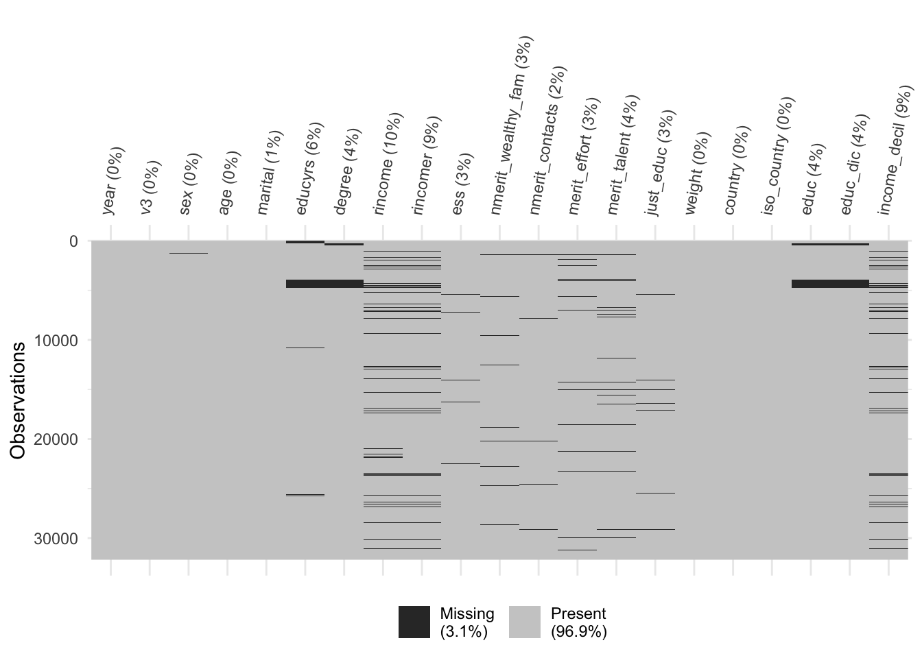
4.4 Save
db_proc99 <- db_proc99 %>%
  select(year, country, iso_country, sex, age, marital, educ, educ_dic, income_decil, ess, just_educ,  merit_effort, merit_talent, nmerit_wealthy_fam, nmerit_contacts, weight)

save(db_proc99, file = here("input/data/proc/db_proc99.RData"))
5 Processing ISSP 2009
5.1 Select
db_proc09 <- issp09 %>%
  janitor::clean_names() %>%
  select(v5,
         sex,
         age,
         marital,
         degree,
         141:181,
         ess = v44,
         nmerit_wealthy_fam = v6,
         nmerit_educated_parents = v7,
         merit_ambition = v9,
         merit_effort = v10,
         nmerit_contacts = v11,
         nmerit_political_connection = v12,
         nmerit_race = v14,
         nmerit_gender = v16,
         just_educ = v39,
         weight
         )
5.2 Recode and transform
5.2.1 Year
db_proc09$year <- 2009
db_proc09$year <- as.numeric(db_proc09$year)
5.2.2 Country
frq(db_proc09$v5)Country (see V4 for codes for the sample) (x) <numeric>
# total N=56021 valid N=56021 mean=432.74 sd=263.79
Value | Label | N | Raw % | Valid % | Cum. %
--------------------------------------------------------------------------------
32 | AR-Argentina | 1133 | 2.02 | 2.02 | 2.02
36 | AU-Australia | 1525 | 2.72 | 2.72 | 4.74
40 | AT-Austria | 1019 | 1.82 | 1.82 | 6.56
56 | BE-Belgium | 1115 | 1.99 | 1.99 | 8.55
100 | BG-Bulgaria | 1000 | 1.79 | 1.79 | 10.34
152 | CL-Chile | 1505 | 2.69 | 2.69 | 13.03
156 | CN-China | 3010 | 5.37 | 5.37 | 18.40
158 | TW-Taiwan | 2026 | 3.62 | 3.62 | 22.01
191 | HR-Croatia | 1201 | 2.14 | 2.14 | 24.16
196 | CY-Cyprus | 1000 | 1.79 | 1.79 | 25.94
203 | CZ-Czech Republic | 1205 | 2.15 | 2.15 | 28.09
208 | DK-Denmark | 1518 | 2.71 | 2.71 | 30.80
233 | EE-Estonia | 1005 | 1.79 | 1.79 | 32.60
246 | FI-Finland | 880 | 1.57 | 1.57 | 34.17
250 | FR-France | 2817 | 5.03 | 5.03 | 39.20
276 | DE-Germany | 1395 | 2.49 | 2.49 | 41.69
348 | HU-Hungary | 1010 | 1.80 | 1.80 | 43.49
352 | IS-Iceland | 947 | 1.69 | 1.69 | 45.18
376 | IL-Israel | 1193 | 2.13 | 2.13 | 47.31
380 | IT-Italy | 1084 | 1.93 | 1.93 | 49.25
392 | JP-Japan | 1296 | 2.31 | 2.31 | 51.56
410 | KR-South Korea | 1599 | 2.85 | 2.85 | 54.41
428 | LV-Latvia | 1069 | 1.91 | 1.91 | 56.32
440 | LT-Lithuania | 1023 | 1.83 | 1.83 | 58.15
554 | NZ-New Zealand | 935 | 1.67 | 1.67 | 59.82
578 | NO-Norway | 1246 | 2.22 | 2.22 | 62.04
608 | PH-Philippines | 1200 | 2.14 | 2.14 | 64.18
616 | PL-Poland | 1263 | 2.25 | 2.25 | 66.44
620 | PT-Portugal | 1000 | 1.79 | 1.79 | 68.22
643 | RU-Russia | 1603 | 2.86 | 2.86 | 71.08
703 | SK-Slovakia | 1159 | 2.07 | 2.07 | 73.15
705 | SI-Slovenia | 1065 | 1.90 | 1.90 | 75.05
710 | ZA-South Africa | 3305 | 5.90 | 5.90 | 80.95
724 | ES-Spain | 1215 | 2.17 | 2.17 | 83.12
752 | SE-Sweden | 1137 | 2.03 | 2.03 | 85.15
756 | CH-Switzerland | 1229 | 2.19 | 2.19 | 87.35
792 | TR-Turkey | 1569 | 2.80 | 2.80 | 90.15
804 | UA-Ukraine | 2012 | 3.59 | 3.59 | 93.74
826 | GB-Great Britain and/or United Kingdom | 958 | 1.71 | 1.71 | 95.45
840 | US-United States | 1581 | 2.82 | 2.82 | 98.27
862 | VE-Venezuela | 969 | 1.73 | 1.73 | 100.00
<NA> | <NA> | 0 | 0.00 | <NA> | <NA>db_proc09$country <- NA
db_proc09$country <- countrycode::countrycode(db_proc09$v5,
origin = "iso3n",
destination = "country.name")
db_proc09$iso_country <- countrycode::countrycode(db_proc09$country,
origin = "country.name",
destination = "iso3c")
frq(db_proc09$country); frq(db_proc09$iso_country)x <character>
# total N=56021 valid N=56021 mean=21.39 sd=11.98
Value | N | Raw % | Valid % | Cum. %
------------------------------------------------
Argentina | 1133 | 2.02 | 2.02 | 2.02
Australia | 1525 | 2.72 | 2.72 | 4.74
Austria | 1019 | 1.82 | 1.82 | 6.56
Belgium | 1115 | 1.99 | 1.99 | 8.55
Bulgaria | 1000 | 1.79 | 1.79 | 10.34
Chile | 1505 | 2.69 | 2.69 | 13.03
China | 3010 | 5.37 | 5.37 | 18.40
Croatia | 1201 | 2.14 | 2.14 | 20.54
Cyprus | 1000 | 1.79 | 1.79 | 22.33
Czechia | 1205 | 2.15 | 2.15 | 24.48
Denmark | 1518 | 2.71 | 2.71 | 27.19
Estonia | 1005 | 1.79 | 1.79 | 28.98
Finland | 880 | 1.57 | 1.57 | 30.55
France | 2817 | 5.03 | 5.03 | 35.58
Germany | 1395 | 2.49 | 2.49 | 38.07
Hungary | 1010 | 1.80 | 1.80 | 39.87
Iceland | 947 | 1.69 | 1.69 | 41.56
Israel | 1193 | 2.13 | 2.13 | 43.69
Italy | 1084 | 1.93 | 1.93 | 45.63
Japan | 1296 | 2.31 | 2.31 | 47.94
Latvia | 1069 | 1.91 | 1.91 | 49.85
Lithuania | 1023 | 1.83 | 1.83 | 51.68
New Zealand | 935 | 1.67 | 1.67 | 53.35
Norway | 1246 | 2.22 | 2.22 | 55.57
Philippines | 1200 | 2.14 | 2.14 | 57.71
Poland | 1263 | 2.25 | 2.25 | 59.97
Portugal | 1000 | 1.79 | 1.79 | 61.75
Russia | 1603 | 2.86 | 2.86 | 64.61
Slovakia | 1159 | 2.07 | 2.07 | 66.68
Slovenia | 1065 | 1.90 | 1.90 | 68.58
South Africa | 3305 | 5.90 | 5.90 | 74.48
South Korea | 1599 | 2.85 | 2.85 | 77.34
Spain | 1215 | 2.17 | 2.17 | 79.51
Sweden | 1137 | 2.03 | 2.03 | 81.54
Switzerland | 1229 | 2.19 | 2.19 | 83.73
Taiwan | 2026 | 3.62 | 3.62 | 87.35
Turkey | 1569 | 2.80 | 2.80 | 90.15
Ukraine | 2012 | 3.59 | 3.59 | 93.74
United Kingdom | 958 | 1.71 | 1.71 | 95.45
United States | 1581 | 2.82 | 2.82 | 98.27
Venezuela | 969 | 1.73 | 1.73 | 100.00
<NA> | 0 | 0.00 | <NA> | <NA>x <character>
# total N=56021 valid N=56021 mean=21.79 sd=12.39
Value | N | Raw % | Valid % | Cum. %
---------------------------------------
ARG | 1133 | 2.02 | 2.02 | 2.02
AUS | 1525 | 2.72 | 2.72 | 4.74
AUT | 1019 | 1.82 | 1.82 | 6.56
BEL | 1115 | 1.99 | 1.99 | 8.55
BGR | 1000 | 1.79 | 1.79 | 10.34
CHE | 1229 | 2.19 | 2.19 | 12.53
CHL | 1505 | 2.69 | 2.69 | 15.22
CHN | 3010 | 5.37 | 5.37 | 20.59
CYP | 1000 | 1.79 | 1.79 | 22.38
CZE | 1205 | 2.15 | 2.15 | 24.53
DEU | 1395 | 2.49 | 2.49 | 27.02
DNK | 1518 | 2.71 | 2.71 | 29.73
ESP | 1215 | 2.17 | 2.17 | 31.90
EST | 1005 | 1.79 | 1.79 | 33.69
FIN | 880 | 1.57 | 1.57 | 35.26
FRA | 2817 | 5.03 | 5.03 | 40.29
GBR | 958 | 1.71 | 1.71 | 42.00
HRV | 1201 | 2.14 | 2.14 | 44.14
HUN | 1010 | 1.80 | 1.80 | 45.95
ISL | 947 | 1.69 | 1.69 | 47.64
ISR | 1193 | 2.13 | 2.13 | 49.77
ITA | 1084 | 1.93 | 1.93 | 51.70
JPN | 1296 | 2.31 | 2.31 | 54.02
KOR | 1599 | 2.85 | 2.85 | 56.87
LTU | 1023 | 1.83 | 1.83 | 58.70
LVA | 1069 | 1.91 | 1.91 | 60.60
NOR | 1246 | 2.22 | 2.22 | 62.83
NZL | 935 | 1.67 | 1.67 | 64.50
PHL | 1200 | 2.14 | 2.14 | 66.64
POL | 1263 | 2.25 | 2.25 | 68.89
PRT | 1000 | 1.79 | 1.79 | 70.68
RUS | 1603 | 2.86 | 2.86 | 73.54
SVK | 1159 | 2.07 | 2.07 | 75.61
SVN | 1065 | 1.90 | 1.90 | 77.51
SWE | 1137 | 2.03 | 2.03 | 79.54
TUR | 1569 | 2.80 | 2.80 | 82.34
TWN | 2026 | 3.62 | 3.62 | 85.96
UKR | 2012 | 3.59 | 3.59 | 89.55
USA | 1581 | 2.82 | 2.82 | 92.37
VEN | 969 | 1.73 | 1.73 | 94.10
ZAF | 3305 | 5.90 | 5.90 | 100.00
<NA> | 0 | 0.00 | <NA> | <NA>5.2.3 Sex
frq(db_proc09$sex)R: Sex (x) <numeric>
# total N=56021 valid N=56021 mean=1.56 sd=0.54
Value | Label | N | Raw % | Valid % | Cum. %
------------------------------------------------------
1 | Male | 25184 | 44.95 | 44.95 | 44.95
2 | Female | 30792 | 54.97 | 54.97 | 99.92
9 | NA, refused | 45 | 0.08 | 0.08 | 100.00
<NA> | <NA> | 0 | 0.00 | <NA> | <NA>db_proc09$sex <- set_na(db_proc09$sex, na = c(9), drop.levels = F)
db_proc09 <- db_proc09 %>%
mutate(sex = if_else(sex == 1, 'Male', 'Female'),
sex = factor(sex, levels = c("Male", "Female")))
frq(db_proc09$sex)x <categorical>
# total N=56021 valid N=55976 mean=1.55 sd=0.50
Value | N | Raw % | Valid % | Cum. %
-----------------------------------------
Male | 25184 | 44.95 | 44.99 | 44.99
Female | 30792 | 54.97 | 55.01 | 100.00
<NA> | 45 | 0.08 | <NA> | <NA>5.2.4 Age
summary(db_proc09$age) Min. 1st Qu. Median Mean 3rd Qu. Max.
15.00 33.00 46.00 46.88 60.00 99.00 db_proc09$age <- set_na(db_proc09$age, na = c(99), drop.levels = F)
db_proc09$age <- as.numeric(db_proc09$age)5.2.5 Marital status
frq(db_proc09$marital)R: Marital status (x) <numeric>
# total N=56021 valid N=56021 mean=2.38 sd=1.81
Value | Label | N | Raw %
------------------------------------------------------------------------------
1 | Married | 31321 | 55.91
2 | Widowed | 4873 | 8.70
3 | Divorced | 3888 | 6.94
4 | Separated (married but sep./not living w legal spouse) | 1052 | 1.88
5 | Never married, single | 14435 | 25.77
9 | NA, refused | 452 | 0.81
<NA> | <NA> | 0 | 0.00
Value | Valid % | Cum. %
------------------------
1 | 55.91 | 55.91
2 | 8.70 | 64.61
3 | 6.94 | 71.55
4 | 1.88 | 73.43
5 | 25.77 | 99.19
9 | 0.81 | 100.00
<NA> | <NA> | <NA>db_proc09$marital <- set_na(db_proc09$marital, na = c(9), drop.levels = F)
db_proc09 <- db_proc09 %>%
mutate(marital = if_else(marital == 1, "Married", "Not married"),
marital = factor(marital, levels = c("Married", "Not married"))
)
frq(db_proc09$marital)x <categorical>
# total N=56021 valid N=55569 mean=1.44 sd=0.50
Value | N | Raw % | Valid % | Cum. %
----------------------------------------------
Married | 31321 | 55.91 | 56.36 | 56.36
Not married | 24248 | 43.28 | 43.64 | 100.00
<NA> | 452 | 0.81 | <NA> | <NA>5.2.6 Education
frq(db_proc09$degree)R: Education II-highest education level (x) <numeric>
# total N=56021 valid N=56021 mean=2.87 sd=1.53
Value | Label | N | Raw %
-------------------------------------------------------------------------
0 | No formal qualification | 2824 | 5.04
1 | Lowest formal qualification | 8847 | 15.79
2 | Above lowest qualification | 10980 | 19.60
3 | Higher secondary completed | 14786 | 26.39
4 | Above higher secondary level, other qualification | 8632 | 15.41
5 | University degree completed | 9565 | 17.07
8 | Dont know | 15 | 0.03
9 | NA | 372 | 0.66
<NA> | <NA> | 0 | 0.00
Value | Valid % | Cum. %
------------------------
0 | 5.04 | 5.04
1 | 15.79 | 20.83
2 | 19.60 | 40.43
3 | 26.39 | 66.83
4 | 15.41 | 82.24
5 | 17.07 | 99.31
8 | 0.03 | 99.34
9 | 0.66 | 100.00
<NA> | <NA> | <NA>db_proc09$degree <- set_na(db_proc09$degree, na = c(8,9), drop.levels = F)
db_proc09 <- db_proc09 %>%
mutate(educ = case_when(degree == 0 ~ "Incomplete primary or less",
degree == 1 ~ "Complete primary",
degree == 2 ~ "Incomplete secondary",
degree == 3 ~ "Complete secondary",
degree == 4 ~ "Incomplete university",
degree == 5 ~ "Complete university",
TRUE ~ NA_character_),
educ = factor(educ,
levels = c("Incomplete primary or less",
"Complete primary",
"Incomplete secondary",
"Complete secondary",
"Incomplete university",
"Complete university")))
db_proc09 <- db_proc09 %>%
mutate(educ_dic = case_when(degree %in% c(0:4) ~ 'Less than universitary',
degree == 5 ~ 'Universitary',
TRUE ~ NA_character_),
educ_dic = factor(educ_dic, levels = c("Universitary", "Less than universitary")))
frq(db_proc09$educ)x <categorical>
# total N=56021 valid N=55634 mean=3.83 sd=1.45
Value | N | Raw % | Valid % | Cum. %
-------------------------------------------------------------
Incomplete primary or less | 2824 | 5.04 | 5.08 | 5.08
Complete primary | 8847 | 15.79 | 15.90 | 20.98
Incomplete secondary | 10980 | 19.60 | 19.74 | 40.71
Complete secondary | 14786 | 26.39 | 26.58 | 67.29
Incomplete university | 8632 | 15.41 | 15.52 | 82.81
Complete university | 9565 | 17.07 | 17.19 | 100.00
<NA> | 387 | 0.69 | <NA> | <NA>frq(db_proc09$educ_dic)x <categorical>
# total N=56021 valid N=55634 mean=1.83 sd=0.38
Value | N | Raw % | Valid % | Cum. %
---------------------------------------------------------
Universitary | 9565 | 17.07 | 17.19 | 17.19
Less than universitary | 46069 | 82.24 | 82.81 | 100.00
<NA> | 387 | 0.69 | <NA> | <NA>5.2.7 Income
#frq(db_proc09$ar_rinc)
#frq(db_proc09$at_rinc)
#frq(db_proc09$au_rinc)
#frq(db_proc09$be_rinc)
#frq(db_proc09$bg_rinc)
#frq(db_proc09$ch_rinc)
#frq(db_proc09$cl_rinc)
#frq(db_proc09$cn_rinc)
#frq(db_proc09$cy_rinc)
#frq(db_proc09$cz_rinc)
#frq(db_proc09$de_rinc)
#frq(db_proc09$dk_rinc)
#frq(db_proc09$ee_rinc)
#frq(db_proc09$es_rinc)
#frq(db_proc09$fi_rinc)
#frq(db_proc09$fr_rinc)
#frq(db_proc09$gb_rinc)
#frq(db_proc09$hr_rinc)
#frq(db_proc09$hu_rinc)
#frq(db_proc09$il_rinc)
#frq(db_proc09$is_rinc)
#frq(db_proc09$it_rinc)
#frq(db_proc09$jp_rinc)
#frq(db_proc09$kr_rinc)
#frq(db_proc09$lt_rinc)
#frq(db_proc09$lv_rinc)
#frq(db_proc09$no_rinc)
#frq(db_proc09$nz_rinc)
#frq(db_proc09$ph_rinc)
#frq(db_proc09$pl_rinc)
#frq(db_proc09$pt_rinc)
#frq(db_proc09$ru_rinc)
#frq(db_proc09$se_rinc)
#frq(db_proc09$si_rinc)
#frq(db_proc09$sk_rinc)
#frq(db_proc09$tr_rinc)
#frq(db_proc09$tw_rinc)
#frq(db_proc09$ua_rinc)
#frq(db_proc09$us_rinc)
#frq(db_proc09$ve_rinc)
#frq(db_proc09$za_rinc)

# ntile function without NAs
ntile_zero_na <- function(x, n = 10) {
  out   <- rep(NA_real_, length(x))
  is_na <- is.na(x)
  is0   <- !is_na & x == 0
  pos   <- !is_na & x > 0
  out[is0] <- 0
  if (any(pos)) out[pos] <- ntile(x[pos], n)
  out
}

db_proc09 <- db_proc09 %>%
 mutate_at(vars(6:46), ~ as.numeric(.)) %>%
  mutate_at(vars(6:46), funs(car::recode(. ,"999990 = NA; 999997 = NA; 999998 = NA; 999999 = NA;
                                              9999990 = NA; 9999997 = NA; 9999998 = NA; 9999999 = NA;
                                              99999990 = NA; 99999997 = NA; 99999998 = NA; 99999999 = NA"))) %>%
  mutate(
    income_personal = do.call(coalesce, across(6:46)),
    income_decil    = ntile_zero_na(income_personal, 10)
  )

db_proc09 %>%
  mutate(n_non_na = rowSums(!is.na(pick(6:46)))) %>%
  count(n_non_na)
# A tibble: 2 × 2
n_non_na n
<dbl> <int>
1 0 8298
2 1 47723frq(db_proc09$income_decil)x <numeric>
# total N=56021 valid N=47723 mean=4.58 sd=3.33
Value | N | Raw % | Valid % | Cum. %
---------------------------------------
0 | 7945 | 14.18 | 16.65 | 16.65
1 | 3978 | 7.10 | 8.34 | 24.98
2 | 3978 | 7.10 | 8.34 | 33.32
3 | 3978 | 7.10 | 8.34 | 41.65
4 | 3978 | 7.10 | 8.34 | 49.99
5 | 3978 | 7.10 | 8.34 | 58.33
6 | 3978 | 7.10 | 8.34 | 66.66
7 | 3978 | 7.10 | 8.34 | 75.00
8 | 3978 | 7.10 | 8.34 | 83.33
9 | 3977 | 7.10 | 8.33 | 91.67
10 | 3977 | 7.10 | 8.33 | 100.00
<NA> | 8298 | 14.81 | <NA> | <NA>5.2.9 Meritocratic variables
frq(db_proc09$merit_effort)Q1e Getting ahead: How important is hard work? (x) <numeric>
# total N=56021 valid N=56021 mean=2.07 sd=1.13
Value | Label | N | Raw % | Valid % | Cum. %
---------------------------------------------------------------
1 | Essential | 17432 | 31.12 | 31.12 | 31.12
2 | Very important | 24403 | 43.56 | 43.56 | 74.68
3 | Fairly important | 10568 | 18.86 | 18.86 | 93.54
4 | Not very important | 2370 | 4.23 | 4.23 | 97.77
5 | Not important at all | 539 | 0.96 | 0.96 | 98.73
8 | Cant choose | 387 | 0.69 | 0.69 | 99.43
9 | NA | 322 | 0.57 | 0.57 | 100.00
<NA> | <NA> | 0 | 0.00 | <NA> | <NA>frq(db_proc09$merit_ambition)Q1d Getting ahead: How Important is having ambition? (x) <numeric>
# total N=56021 valid N=56021 mean=2.22 sd=1.25
Value | Label | N | Raw % | Valid % | Cum. %
---------------------------------------------------------------
1 | Essential | 15238 | 27.20 | 27.20 | 27.20
2 | Very important | 23618 | 42.16 | 42.16 | 69.36
3 | Fairly important | 12124 | 21.64 | 21.64 | 91.00
4 | Not very important | 2950 | 5.27 | 5.27 | 96.27
5 | Not important at all | 1030 | 1.84 | 1.84 | 98.11
8 | Cant choose | 761 | 1.36 | 1.36 | 99.46
9 | NA | 300 | 0.54 | 0.54 | 100.00
<NA> | <NA> | 0 | 0.00 | <NA> | <NA>db_proc09 <- db_proc09 %>%
mutate(
across(
.cols = c(merit_effort, merit_ambition),
.fns = ~ set_na(., na = c(8,9), drop.levels = F)
)
) # ok
db_proc09$merit_effort <- sjmisc::rec(db_proc09$merit_effort,rec = "rev")
db_proc09$merit_ambition <- sjmisc::rec(db_proc09$merit_ambition,rec = "rev")
frq(db_proc09$merit_effort)Q1e Getting ahead: How important is hard work? (x) <numeric>
# total N=56021 valid N=55312 mean=4.01 sd=0.87
Value | Label | N | Raw % | Valid % | Cum. %
---------------------------------------------------------------
1 | Not important at all | 539 | 0.96 | 0.97 | 0.97
2 | Not very important | 2370 | 4.23 | 4.28 | 5.26
3 | Fairly important | 10568 | 18.86 | 19.11 | 24.37
4 | Very important | 24403 | 43.56 | 44.12 | 68.48
5 | Essential | 17432 | 31.12 | 31.52 | 100.00
<NA> | <NA> | 709 | 1.27 | <NA> | <NA>frq(db_proc09$merit_ambition)Q1d Getting ahead: How Important is having ambition? (x) <numeric>
# total N=56021 valid N=54960 mean=3.89 sd=0.93
Value | Label | N | Raw % | Valid % | Cum. %
---------------------------------------------------------------
1 | Not important at all | 1030 | 1.84 | 1.87 | 1.87
2 | Not very important | 2950 | 5.27 | 5.37 | 7.24
3 | Fairly important | 12124 | 21.64 | 22.06 | 29.30
4 | Very important | 23618 | 42.16 | 42.97 | 72.27
5 | Essential | 15238 | 27.20 | 27.73 | 100.00
<NA> | <NA> | 1061 | 1.89 | <NA> | <NA>5.2.10 Non-meritocratic variables
frq(db_proc09$nmerit_wealthy_fam)Q1a Getting ahead: How important is coming from a wealthy family? (x) <numeric>
# total N=56021 valid N=56021 mean=3.19 sd=1.37
Value | Label | N | Raw % | Valid % | Cum. %
---------------------------------------------------------------
1 | Essential | 5256 | 9.38 | 9.38 | 9.38
2 | Very important | 12554 | 22.41 | 22.41 | 31.79
3 | Fairly important | 15782 | 28.17 | 28.17 | 59.96
4 | Not very important | 14609 | 26.08 | 26.08 | 86.04
5 | Not important at all | 6675 | 11.92 | 11.92 | 97.96
8 | Cant choose | 842 | 1.50 | 1.50 | 99.46
9 | NA | 303 | 0.54 | 0.54 | 100.00
<NA> | <NA> | 0 | 0.00 | <NA> | <NA>frq(db_proc09$nmerit_contacts)Q1f Getting ahead: How important is knowing the right people? (x) <numeric>
# total N=56021 valid N=56021 mean=2.56 sd=1.28
Value | Label | N | Raw % | Valid % | Cum. %
---------------------------------------------------------------
1 | Essential | 10029 | 17.90 | 17.90 | 17.90
2 | Very important | 20089 | 35.86 | 35.86 | 53.76
3 | Fairly important | 16847 | 30.07 | 30.07 | 83.83
4 | Not very important | 6379 | 11.39 | 11.39 | 95.22
5 | Not important at all | 1622 | 2.90 | 2.90 | 98.12
8 | Cant choose | 727 | 1.30 | 1.30 | 99.41
9 | NA | 328 | 0.59 | 0.59 | 100.00
<NA> | <NA> | 0 | 0.00 | <NA> | <NA>frq(db_proc09$nmerit_educated_parents)Q1b Getting ahead: How important is having well-educated parents? (x) <numeric>
# total N=56021 valid N=56021 mean=2.85 sd=1.26
Value | Label | N | Raw % | Valid % | Cum. %
---------------------------------------------------------------
1 | Essential | 5975 | 10.67 | 10.67 | 10.67
2 | Very important | 17720 | 31.63 | 31.63 | 42.30
3 | Fairly important | 18221 | 32.53 | 32.53 | 74.82
4 | Not very important | 9905 | 17.68 | 17.68 | 92.50
5 | Not important at all | 3329 | 5.94 | 5.94 | 98.45
8 | Cant choose | 565 | 1.01 | 1.01 | 99.45
9 | NA | 306 | 0.55 | 0.55 | 100.00
<NA> | <NA> | 0 | 0.00 | <NA> | <NA>frq(db_proc09$nmerit_political_connection)Q1g Getting ahead: How important is having political connections? (x) <numeric>
# total N=56021 valid N=56021 mean=3.59 sd=1.59
Value | Label | N | Raw % | Valid % | Cum. %
---------------------------------------------------------------
1 | Essential | 4461 | 7.96 | 7.96 | 7.96
2 | Very important | 9164 | 16.36 | 16.36 | 24.32
3 | Fairly important | 13103 | 23.39 | 23.39 | 47.71
4 | Not very important | 16560 | 29.56 | 29.56 | 77.27
5 | Not important at all | 9811 | 17.51 | 17.51 | 94.78
8 | Cant choose | 2490 | 4.44 | 4.44 | 99.23
9 | NA | 432 | 0.77 | 0.77 | 100.00
<NA> | <NA> | 0 | 0.00 | <NA> | <NA>frq(db_proc09$nmerit_race)Q1i Getting ahead: How important is a person's race? (x) <numeric>
# total N=56021 valid N=56021 mean=4.00 sd=1.46
Value | Label | N | Raw % | Valid % | Cum. %
---------------------------------------------------------------
1 | Essential | 2092 | 3.73 | 3.73 | 3.73
2 | Very important | 6277 | 11.20 | 11.20 | 14.94
3 | Fairly important | 10772 | 19.23 | 19.23 | 34.17
4 | Not very important | 15745 | 28.11 | 28.11 | 62.27
5 | Not important at all | 18566 | 33.14 | 33.14 | 95.41
8 | Cant choose | 2012 | 3.59 | 3.59 | 99.01
9 | NA | 557 | 0.99 | 0.99 | 100.00
<NA> | <NA> | 0 | 0.00 | <NA> | <NA>frq(db_proc09$nmerit_gender)Q1k Getting ahead: How important is being born a man or a woman? (x) <numeric>
# total N=56021 valid N=56021 mean=3.99 sd=1.45
Value | Label | N | Raw % | Valid % | Cum. %
---------------------------------------------------------------
1 | Essential | 2241 | 4.00 | 4.00 | 4.00
2 | Very important | 6197 | 11.06 | 11.06 | 15.06
3 | Fairly important | 10644 | 19.00 | 19.00 | 34.06
4 | Not very important | 15789 | 28.18 | 28.18 | 62.25
5 | Not important at all | 18694 | 33.37 | 33.37 | 95.62
8 | Cant choose | 2010 | 3.59 | 3.59 | 99.20
9 | NA | 446 | 0.80 | 0.80 | 100.00
<NA> | <NA> | 0 | 0.00 | <NA> | <NA>db_proc09 <- db_proc09 %>%
mutate(
across(
.cols = c(nmerit_wealthy_fam, nmerit_contacts, nmerit_educated_parents,
nmerit_political_connection, nmerit_race, nmerit_gender),
.fns = ~ set_na(., na = c(8,9), drop.levels = F)
)
) # ok
db_proc09$nmerit_wealthy_fam <- sjmisc::rec(db_proc09$nmerit_wealthy_fam,rec = "rev")
db_proc09$nmerit_contacts <- sjmisc::rec(db_proc09$nmerit_contacts,rec = "rev")
db_proc09$nmerit_educated_parents <- sjmisc::rec(db_proc09$nmerit_educated_parents,rec = "rev")
db_proc09$nmerit_political_connection <- sjmisc::rec(db_proc09$nmerit_political_connection,rec = "rev")
db_proc09$nmerit_race <- sjmisc::rec(db_proc09$nmerit_race,rec = "rev")
db_proc09$nmerit_gender <- sjmisc::rec(db_proc09$nmerit_gender,rec = "rev")
frq(db_proc09$nmerit_wealthy_fam)Q1a Getting ahead: How important is coming from a wealthy family? (x) <numeric>
# total N=56021 valid N=54876 mean=2.91 sd=1.16
Value | Label | N | Raw % | Valid % | Cum. %
---------------------------------------------------------------
1 | Not important at all | 6675 | 11.92 | 12.16 | 12.16
2 | Not very important | 14609 | 26.08 | 26.62 | 38.79
3 | Fairly important | 15782 | 28.17 | 28.76 | 67.55
4 | Very important | 12554 | 22.41 | 22.88 | 90.42
5 | Essential | 5256 | 9.38 | 9.58 | 100.00
<NA> | <NA> | 1145 | 2.04 | <NA> | <NA>frq(db_proc09$nmerit_contacts)Q1f Getting ahead: How important is knowing the right people? (x) <numeric>
# total N=56021 valid N=54966 mean=3.56 sd=1.01
Value | Label | N | Raw % | Valid % | Cum. %
---------------------------------------------------------------
1 | Not important at all | 1622 | 2.90 | 2.95 | 2.95
2 | Not very important | 6379 | 11.39 | 11.61 | 14.56
3 | Fairly important | 16847 | 30.07 | 30.65 | 45.21
4 | Very important | 20089 | 35.86 | 36.55 | 81.75
5 | Essential | 10029 | 17.90 | 18.25 | 100.00
<NA> | <NA> | 1055 | 1.88 | <NA> | <NA>frq(db_proc09$nmerit_educated_parents)Q1b Getting ahead: How important is having well-educated parents? (x) <numeric>
# total N=56021 valid N=55150 mean=3.24 sd=1.06
Value | Label | N | Raw % | Valid % | Cum. %
---------------------------------------------------------------
1 | Not important at all | 3329 | 5.94 | 6.04 | 6.04
2 | Not very important | 9905 | 17.68 | 17.96 | 24.00
3 | Fairly important | 18221 | 32.53 | 33.04 | 57.04
4 | Very important | 17720 | 31.63 | 32.13 | 89.17
5 | Essential | 5975 | 10.67 | 10.83 | 100.00
<NA> | <NA> | 871 | 1.55 | <NA> | <NA>frq(db_proc09$nmerit_political_connection)Q1g Getting ahead: How important is having political connections? (x) <numeric>
# total N=56021 valid N=53099 mean=2.66 sd=1.20
Value | Label | N | Raw % | Valid % | Cum. %
---------------------------------------------------------------
1 | Not important at all | 9811 | 17.51 | 18.48 | 18.48
2 | Not very important | 16560 | 29.56 | 31.19 | 49.66
3 | Fairly important | 13103 | 23.39 | 24.68 | 74.34
4 | Very important | 9164 | 16.36 | 17.26 | 91.60
5 | Essential | 4461 | 7.96 | 8.40 | 100.00
<NA> | <NA> | 2922 | 5.22 | <NA> | <NA>frq(db_proc09$nmerit_race)Q1i Getting ahead: How important is a person's race? (x) <numeric>
# total N=56021 valid N=53452 mean=2.21 sd=1.15
Value | Label | N | Raw % | Valid % | Cum. %
---------------------------------------------------------------
1 | Not important at all | 18566 | 33.14 | 34.73 | 34.73
2 | Not very important | 15745 | 28.11 | 29.46 | 64.19
3 | Fairly important | 10772 | 19.23 | 20.15 | 84.34
4 | Very important | 6277 | 11.20 | 11.74 | 96.09
5 | Essential | 2092 | 3.73 | 3.91 | 100.00
<NA> | <NA> | 2569 | 4.59 | <NA> | <NA>frq(db_proc09$nmerit_gender)Q1k Getting ahead: How important is being born a man or a woman? (x) <numeric>
# total N=56021 valid N=53565 mean=2.21 sd=1.16
Value | Label | N | Raw % | Valid % | Cum. %
---------------------------------------------------------------
1 | Not important at all | 18694 | 33.37 | 34.90 | 34.90
2 | Not very important | 15789 | 28.18 | 29.48 | 64.38
3 | Fairly important | 10644 | 19.00 | 19.87 | 84.25
4 | Very important | 6197 | 11.06 | 11.57 | 95.82
5 | Essential | 2241 | 4.00 | 4.18 | 100.00
<NA> | <NA> | 2456 | 4.38 | <NA> | <NA>5.2.11 Market justice in education
frq(db_proc09$just_educ)Q8b Just or unjust - that people with higher incomes can buy better education fo (x) <numeric>
# total N=56021 valid N=56021 mean=3.65 sd=1.55
Value | Label | N | Raw % | Valid % | Cum. %
----------------------------------------------------------------------------------
1 | Very just, definitely right | 4793 | 8.56 | 8.56 | 8.56
2 | Somewhat just, right | 9805 | 17.50 | 17.50 | 26.06
3 | Neither just nor unjust, mixed feelings | 9531 | 17.01 | 17.01 | 43.07
4 | Somewhat unjust, wrong | 13763 | 24.57 | 24.57 | 67.64
5 | Very unjust, definitely wrong | 16328 | 29.15 | 29.15 | 96.79
8 | Cant choose | 1401 | 2.50 | 2.50 | 99.29
9 | NA | 400 | 0.71 | 0.71 | 100.00
<NA> | <NA> | 0 | 0.00 | <NA> | <NA>db_proc09$just_educ <- set_na(db_proc09$just_educ, na = c(8,9), drop.levels = F)
db_proc09$just_educ <- sjmisc::rec(db_proc09$just_educ,rec = "rev")
frq(db_proc09$just_educ)Q8b Just or unjust - that people with higher incomes can buy better education fo (x) <numeric>
# total N=56021 valid N=54220 mean=2.50 sd=1.32
Value | Label | N | Raw % | Valid % | Cum. %
----------------------------------------------------------------------------------
1 | Very unjust, definitely wrong | 16328 | 29.15 | 30.11 | 30.11
2 | Somewhat unjust, wrong | 13763 | 24.57 | 25.38 | 55.50
3 | Neither just nor unjust, mixed feelings | 9531 | 17.01 | 17.58 | 73.08
4 | Somewhat just, right | 9805 | 17.50 | 18.08 | 91.16
5 | Very just, definitely right | 4793 | 8.56 | 8.84 | 100.00
<NA> | <NA> | 1801 | 3.21 | <NA> | <NA>5.3 Missing values
db_proc09 <- db_proc09 %>%
  select(year, country, iso_country, sex, age, marital, educ, educ_dic, income_decil, ess, just_educ, merit_effort, merit_ambition, nmerit_wealthy_fam, nmerit_contacts, nmerit_educated_parents, nmerit_political_connection, nmerit_race, nmerit_gender, weight)

colSums(is.na(db_proc09))
year country
0 0
iso_country sex
0 45
age marital
138 452
educ educ_dic
387 387
income_decil ess
8298 884
just_educ merit_effort
1801 709
merit_ambition nmerit_wealthy_fam
1061 1145
nmerit_contacts nmerit_educated_parents
1055 871
nmerit_political_connection nmerit_race
2922 2569
nmerit_gender weight
2456 0 n_miss(db_proc09)[1] 25180prop_miss(db_proc09)*100[1] 2.247372miss_var_summary(db_proc09)# A tibble: 20 × 3
variable n_miss pct_miss
<chr> <int> <num>
1 income_decil 8298 14.8
2 nmerit_political_connection 2922 5.22
3 nmerit_race 2569 4.59
4 nmerit_gender 2456 4.38
5 just_educ 1801 3.21
6 nmerit_wealthy_fam 1145 2.04
7 merit_ambition 1061 1.89
8 nmerit_contacts 1055 1.88
9 ess 884 1.58
10 nmerit_educated_parents 871 1.55
11 merit_effort 709 1.27
12 marital 452 0.807
13 educ 387 0.691
14 educ_dic 387 0.691
15 age 138 0.246
16 sex 45 0.0803
17 year 0 0
18 country 0 0
19 iso_country 0 0
20 weight 0 0 vis_miss(db_proc09, warn_large_data = F) + theme(axis.text.x = element_text(angle=80))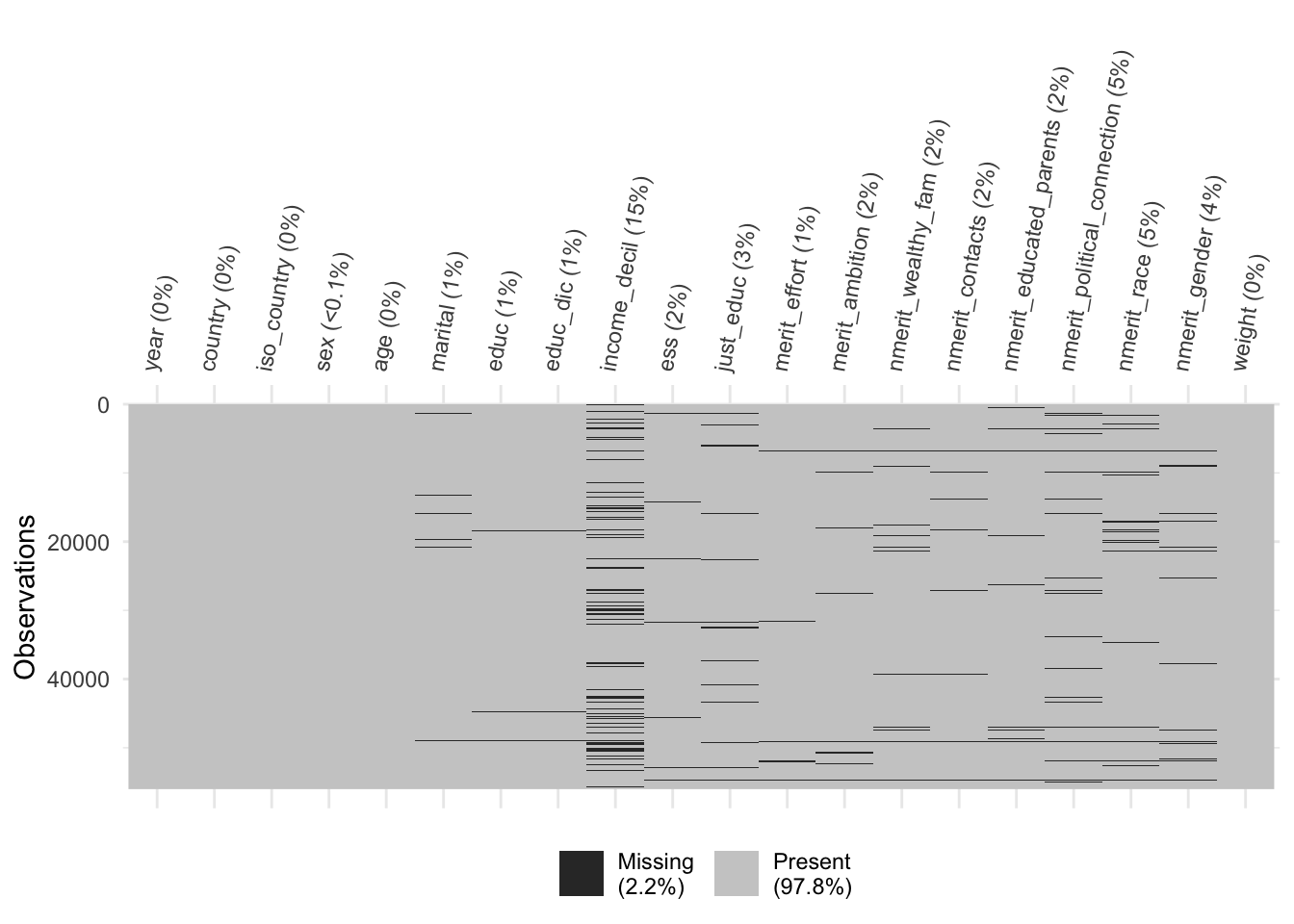
5.4 Save
save(db_proc09, file = here("input/data/proc/db_proc09.RData"))6 Processing ISSP 2019
6.1 Select
db_proc19 <- issp19 %>%
  janitor::clean_names() %>%
  select(country,
         sex,
         age,
         marital,
         degree,
         258:286,
         ess = topbot,
         nmerit_wealthy_fam = v1,
         nmerit_educated_parents = v2,
         merit_effort = v4,
         nmerit_contacts = v5,
         nmerit_political_connection = v6,
         nmerit_race = v8,
         nmerit_gender = v10,
         just_educ = v31,
         weight
         )
6.2 Recode and transform
6.2.1 Year
db_proc19$year <- 2019
db_proc19$year <- as.numeric(db_proc19$year)
6.2.2 Country
frq(db_proc19$country)Country ISO 3166 Code (see c_sample for codes for the sample) (x) <numeric>
# total N=44975 valid N=44975 mean=491.18 sd=258.70
Value | Label | N | Raw % | Valid % | Cum. %
----------------------------------------------------------------
36 | 36. AU-Australia | 1068 | 2.37 | 2.37 | 2.37
40 | 40. AT-Austria | 1261 | 2.80 | 2.80 | 5.18
100 | 100. BG-Bulgaria | 1151 | 2.56 | 2.56 | 7.74
152 | 152. CL-Chile | 1374 | 3.06 | 3.06 | 10.79
158 | 158. TW-Taiwan | 1926 | 4.28 | 4.28 | 15.08
191 | 191. HR-Croatia | 1000 | 2.22 | 2.22 | 17.30
203 | 203. CZ-Czech Republic | 1924 | 4.28 | 4.28 | 21.58
208 | 208. DK-Denmark | 1038 | 2.31 | 2.31 | 23.88
246 | 246. FI-Finland | 966 | 2.15 | 2.15 | 26.03
250 | 250. FR-France | 1598 | 3.55 | 3.55 | 29.59
276 | 276. DE-Germany | 1325 | 2.95 | 2.95 | 32.53
352 | 352. IS-Iceland | 1227 | 2.73 | 2.73 | 35.26
376 | 376. IL-Israel | 1201 | 2.67 | 2.67 | 37.93
380 | 380. IT-Italy | 1215 | 2.70 | 2.70 | 40.63
392 | 392. JP-Japan | 1473 | 3.28 | 3.28 | 43.91
440 | 440. LT-Lithuania | 1050 | 2.33 | 2.33 | 46.24
554 | 554. NZ-New Zealand | 1210 | 2.69 | 2.69 | 48.93
578 | 578. NO-Norway | 1323 | 2.94 | 2.94 | 51.87
608 | 608. PH-Philippines | 4250 | 9.45 | 9.45 | 61.32
643 | 643. RU-Russia | 1597 | 3.55 | 3.55 | 64.87
705 | 705. SI-Slovenia | 1164 | 2.59 | 2.59 | 67.46
710 | 710. ZA-South Africa | 2727 | 6.06 | 6.06 | 73.53
740 | 740. SR-Suriname | 1001 | 2.23 | 2.23 | 75.75
752 | 752. SE-Sweden | 1636 | 3.64 | 3.64 | 79.39
756 | 756. CH-Switzerland | 3042 | 6.76 | 6.76 | 86.15
764 | 764. TH-Thailand | 1533 | 3.41 | 3.41 | 89.56
826 | 826. GB-Great Britain | 1724 | 3.83 | 3.83 | 93.39
840 | 840. US-United States | 1852 | 4.12 | 4.12 | 97.51
862 | 862. VE-Venezuela | 1119 | 2.49 | 2.49 | 100.00
<NA> | <NA> | 0 | 0.00 | <NA> | <NA>db_proc19$country <- countrycode::countrycode(db_proc19$country,
origin = "iso3n",
destination = "country.name")
db_proc19$iso_country <- countrycode::countrycode(db_proc19$country,
origin = "country.name",
destination = "iso3c")
frq(db_proc19$country); frq(db_proc19$iso_country)x <character>
# total N=44975 valid N=44975 mean=16.29 sd=8.08
Value | N | Raw % | Valid % | Cum. %
------------------------------------------------
Australia | 1068 | 2.37 | 2.37 | 2.37
Austria | 1261 | 2.80 | 2.80 | 5.18
Bulgaria | 1151 | 2.56 | 2.56 | 7.74
Chile | 1374 | 3.06 | 3.06 | 10.79
Croatia | 1000 | 2.22 | 2.22 | 13.02
Czechia | 1924 | 4.28 | 4.28 | 17.29
Denmark | 1038 | 2.31 | 2.31 | 19.60
Finland | 966 | 2.15 | 2.15 | 21.75
France | 1598 | 3.55 | 3.55 | 25.30
Germany | 1325 | 2.95 | 2.95 | 28.25
Iceland | 1227 | 2.73 | 2.73 | 30.98
Israel | 1201 | 2.67 | 2.67 | 33.65
Italy | 1215 | 2.70 | 2.70 | 36.35
Japan | 1473 | 3.28 | 3.28 | 39.62
Lithuania | 1050 | 2.33 | 2.33 | 41.96
New Zealand | 1210 | 2.69 | 2.69 | 44.65
Norway | 1323 | 2.94 | 2.94 | 47.59
Philippines | 4250 | 9.45 | 9.45 | 57.04
Russia | 1597 | 3.55 | 3.55 | 60.59
Slovenia | 1164 | 2.59 | 2.59 | 63.18
South Africa | 2727 | 6.06 | 6.06 | 69.24
Suriname | 1001 | 2.23 | 2.23 | 71.47
Sweden | 1636 | 3.64 | 3.64 | 75.11
Switzerland | 3042 | 6.76 | 6.76 | 81.87
Taiwan | 1926 | 4.28 | 4.28 | 86.15
Thailand | 1533 | 3.41 | 3.41 | 89.56
United Kingdom | 1724 | 3.83 | 3.83 | 93.39
United States | 1852 | 4.12 | 4.12 | 97.51
Venezuela | 1119 | 2.49 | 2.49 | 100.00
<NA> | 0 | 0.00 | <NA> | <NA>x <character>
# total N=44975 valid N=44975 mean=15.69 sd=8.59
Value | N | Raw % | Valid % | Cum. %
---------------------------------------
AUS | 1068 | 2.37 | 2.37 | 2.37
AUT | 1261 | 2.80 | 2.80 | 5.18
BGR | 1151 | 2.56 | 2.56 | 7.74
CHE | 3042 | 6.76 | 6.76 | 14.50
CHL | 1374 | 3.06 | 3.06 | 17.56
CZE | 1924 | 4.28 | 4.28 | 21.83
DEU | 1325 | 2.95 | 2.95 | 24.78
DNK | 1038 | 2.31 | 2.31 | 27.09
FIN | 966 | 2.15 | 2.15 | 29.24
FRA | 1598 | 3.55 | 3.55 | 32.79
GBR | 1724 | 3.83 | 3.83 | 36.62
HRV | 1000 | 2.22 | 2.22 | 38.85
ISL | 1227 | 2.73 | 2.73 | 41.57
ISR | 1201 | 2.67 | 2.67 | 44.24
ITA | 1215 | 2.70 | 2.70 | 46.95
JPN | 1473 | 3.28 | 3.28 | 50.22
LTU | 1050 | 2.33 | 2.33 | 52.56
NOR | 1323 | 2.94 | 2.94 | 55.50
NZL | 1210 | 2.69 | 2.69 | 58.19
PHL | 4250 | 9.45 | 9.45 | 67.64
RUS | 1597 | 3.55 | 3.55 | 71.19
SUR | 1001 | 2.23 | 2.23 | 73.41
SVN | 1164 | 2.59 | 2.59 | 76.00
SWE | 1636 | 3.64 | 3.64 | 79.64
THA | 1533 | 3.41 | 3.41 | 83.05
TWN | 1926 | 4.28 | 4.28 | 87.33
USA | 1852 | 4.12 | 4.12 | 91.45
VEN | 1119 | 2.49 | 2.49 | 93.94
ZAF | 2727 | 6.06 | 6.06 | 100.00
<NA> | 0 | 0.00 | <NA> | <NA>6.2.3 Sex
frq(db_proc19$sex)Sex of Respondent (x) <numeric>
# total N=44975 valid N=44975 mean=1.51 sd=0.68
Value | Label | N | Raw % | Valid % | Cum. %
--------------------------------------------------------
-9 | -9. No answer | 85 | 0.19 | 0.19 | 0.19
1 | 1. Male | 20969 | 46.62 | 46.62 | 46.81
2 | 2. Female | 23921 | 53.19 | 53.19 | 100.00
<NA> | <NA> | 0 | 0.00 | <NA> | <NA>db_proc19$sex <- set_na(db_proc19$sex, na = c(-9), drop.levels = F)
db_proc19 <- db_proc19 %>%
mutate(sex = if_else(sex == 1, 'Male', 'Female'),
sex = factor(sex, levels = c("Male", "Female")))
frq(db_proc19$sex)x <categorical>
# total N=44975 valid N=44890 mean=1.53 sd=0.50
Value | N | Raw % | Valid % | Cum. %
-----------------------------------------
Male | 20969 | 46.62 | 46.71 | 46.71
Female | 23921 | 53.19 | 53.29 | 100.00
<NA> | 85 | 0.19 | <NA> | <NA>6.2.4 Age
summary(db_proc19$age) Min. 1st Qu. Median Mean 3rd Qu. Max.
-9.00 35.00 49.00 49.11 63.00 105.00 db_proc19$age <- set_na(db_proc19$age, na = c(-9), drop.levels = F)
db_proc19$age <- as.numeric(db_proc19$age)6.2.5 Marital status
frq(db_proc19$marital)Legal partnership status (x) <numeric>
# total N=44975 valid N=44975 mean=2.87 sd=2.63
Value
-----
-9
-7
1
2
3
4
5
6
<NA>
Label
-----------------------------------------------------------------------------------------------------
-9. No answer
-7. Refused
1. Married
2. Civil partnership
3. Separated from spouse/ civil partner (still legally married/ still legally in a civil partnership)
4. Divorced from spouse/ legally separated from civil partner; AT: Divorced/ Separated
5. Widowed/ civil partner died
6. Never married/ never in a civil partnership
<NA>
N | Raw % | Valid % | Cum. %
--------------------------------
457 | 1.02 | 1.02 | 1.02
232 | 0.52 | 0.52 | 1.53
22688 | 50.45 | 50.45 | 51.98
1080 | 2.40 | 2.40 | 54.38
852 | 1.89 | 1.89 | 56.27
3580 | 7.96 | 7.96 | 64.23
3530 | 7.85 | 7.85 | 72.08
12556 | 27.92 | 27.92 | 100.00
0 | 0.00 | <NA> | <NA>db_proc19$marital <- set_na(db_proc19$marital, na = c(-9, -7), drop.levels = F)
db_proc19 <- db_proc19 %>%
mutate(marital = if_else(marital %in% c(1,2,3), "Married", "Not married"),
marital = factor(marital, levels = c("Married", "Not married"))
)
frq(db_proc19$marital)x <categorical>
# total N=44975 valid N=44975 mean=1.45 sd=0.50
Value | N | Raw % | Valid % | Cum. %
----------------------------------------------
Married | 24620 | 54.74 | 54.74 | 54.74
Not married | 20355 | 45.26 | 45.26 | 100.00
<NA> | 0 | 0.00 | <NA> | <NA>6.2.6 Education
frq(db_proc19$degree)Comparative: highest completed degree of education (derived from nat_DEGR) (x) <numeric>
# total N=44975 valid N=44975 mean=3.32 sd=2.06
Value
-----
-9
0
1
2
3
4
5
6
<NA>
Label
----------------------------------------------------------------------------------------------------------------
-9. No answer
0. No formal education
1. Primary school (elementary education)
2. Lower secondary (secondary completed that does not allow entry to university: end of obligatory school)
3. Upper secondary (programs that allows entry to university)
4. Post secondary, non-tertiary (other upper secondary programs toward the labour market or technical formation)
5. Lower level tertiary, first stage (also technical schools at a tertiary level)
6. Upper level tertiary (Master, Doctor)
<NA>
N | Raw % | Valid % | Cum. %
--------------------------------
487 | 1.08 | 1.08 | 1.08
1647 | 3.66 | 3.66 | 4.74
2946 | 6.55 | 6.55 | 11.30
8853 | 19.68 | 19.68 | 30.98
10833 | 24.09 | 24.09 | 55.07
5854 | 13.02 | 13.02 | 68.08
9089 | 20.21 | 20.21 | 88.29
5266 | 11.71 | 11.71 | 100.00
0 | 0.00 | <NA> | <NA>db_proc19$degree <- set_na(db_proc19$degree, na = c(-9), drop.levels = F)
db_proc19 <- db_proc19 %>%
mutate(educ = case_when(degree == 0 ~ "Incomplete primary or less",
degree == 1 ~ "Complete primary",
degree == 2 ~ "Incomplete secondary",
degree == 3 ~ "Complete secondary",
degree == 4 ~ "Incomplete university",
degree %in% c(5,6) ~ "Complete university",
TRUE ~ NA_character_),
educ = factor(educ,
levels = c("Incomplete primary or less",
"Complete primary",
"Incomplete secondary",
"Complete secondary",
"Incomplete university",
"Complete university")))
db_proc19 <- db_proc19 %>%
mutate(educ_dic = case_when(degree %in% c(0:4) ~ 'Less than universitary',
degree %in% c(5:6) ~ 'Universitary',
TRUE ~ NA_character_),
educ_dic = factor(educ_dic, levels = c("Universitary", "Less than universitary")))
frq(db_proc19$educ)x <categorical>
# total N=44975 valid N=44488 mean=4.33 sd=1.45
Value | N | Raw % | Valid % | Cum. %
-------------------------------------------------------------
Incomplete primary or less | 1647 | 3.66 | 3.70 | 3.70
Complete primary | 2946 | 6.55 | 6.62 | 10.32
Incomplete secondary | 8853 | 19.68 | 19.90 | 30.22
Complete secondary | 10833 | 24.09 | 24.35 | 54.57
Incomplete university | 5854 | 13.02 | 13.16 | 67.73
Complete university | 14355 | 31.92 | 32.27 | 100.00
<NA> | 487 | 1.08 | <NA> | <NA>frq(db_proc19$educ_dic)x <categorical>
# total N=44975 valid N=44488 mean=1.68 sd=0.47
Value | N | Raw % | Valid % | Cum. %
---------------------------------------------------------
Universitary | 14355 | 31.92 | 32.27 | 32.27
Less than universitary | 30133 | 67.00 | 67.73 | 100.00
<NA> | 487 | 1.08 | <NA> | <NA>6.2.7 Income
#frq(db_proc19$at_rinc)
#frq(db_proc19$au_rinc)
#frq(db_proc19$bg_rinc)
#frq(db_proc19$ch_rinc)
#frq(db_proc19$cl_rinc)
#frq(db_proc19$cz_rinc)
#frq(db_proc19$de_rinc)
#frq(db_proc19$dk_rinc)
#frq(db_proc19$fi_rinc)
#frq(db_proc19$fr_rinc)
#frq(db_proc19$gb_rinc)
#frq(db_proc19$hr_rinc)
#frq(db_proc19$il_rinc)
#frq(db_proc19$is_rinc)
#frq(db_proc19$it_rinc)
#frq(db_proc19$jp_rinc)
#frq(db_proc19$lt_rinc)
#frq(db_proc19$no_rinc)
#frq(db_proc19$nz_rinc)
#frq(db_proc19$ph_rinc)
#frq(db_proc19$ru_rinc)
#frq(db_proc19$se_rinc)
#frq(db_proc19$si_rinc)
#frq(db_proc19$sr_rinc)
#frq(db_proc19$th_rinc)
#frq(db_proc19$tw_rinc)
#frq(db_proc19$us_rinc)
#frq(db_proc19$ve_rinc)
#frq(db_proc19$za_rinc)

# ntile function without NAs
ntile_zero_na <- function(x, n = 10) {
  out   <- rep(NA_real_, length(x))
  is_na <- is.na(x)
  is0   <- !is_na & x == 0
  pos   <- !is_na & x > 0
  out[is0] <- 0
  if (any(pos)) out[pos] <- ntile(x[pos], n)
  out
}

db_proc19 <- db_proc19 %>%
  mutate_at(vars(5:34), ~ as.numeric(.)) %>%
 mutate_at(vars(5:34), funs(car::recode(. ,"-9 = NA; -8 = NA; -7 = NA; -2 = NA"))) %>%
  mutate(
    income_personal = do.call(coalesce, across(5:34)),
    income_decil    = ntile_zero_na(income_personal, 10)
  )

db_proc19 %>%
  mutate(n_non_na = rowSums(!is.na(pick(5:34)))) %>%
  count(n_non_na)
# A tibble: 3 × 2
n_non_na n
<dbl> <int>
1 0 218
2 1 5687
3 2 39070frq(db_proc19$income_decil)x <numeric>
# total N=44975 valid N=44757 mean=5.29 sd=3.01
Value | N | Raw % | Valid % | Cum. %
---------------------------------------
0 | 1691 | 3.76 | 3.78 | 3.78
1 | 4307 | 9.58 | 9.62 | 13.40
2 | 4307 | 9.58 | 9.62 | 23.02
3 | 4307 | 9.58 | 9.62 | 32.65
4 | 4307 | 9.58 | 9.62 | 42.27
5 | 4307 | 9.58 | 9.62 | 51.89
6 | 4307 | 9.58 | 9.62 | 61.52
7 | 4306 | 9.57 | 9.62 | 71.14
8 | 4306 | 9.57 | 9.62 | 80.76
9 | 4306 | 9.57 | 9.62 | 90.38
10 | 4306 | 9.57 | 9.62 | 100.00
<NA> | 218 | 0.48 | <NA> | <NA>6.2.9 Meritocratic variables
frq(db_proc19$merit_effort)Q1d Getting ahead: How important is hard work? (x) <numeric>
# total N=44975 valid N=44975 mean=1.89 sd=1.50
Value | Label | N | Raw % | Valid % | Cum. %
------------------------------------------------------------------
-9 | -9. No answer | 270 | 0.60 | 0.60 | 0.60
-8 | -8. Can't choose | 308 | 0.68 | 0.68 | 1.29
1 | 1. Essential | 14264 | 31.72 | 31.72 | 33.00
2 | 2. Very important | 18246 | 40.57 | 40.57 | 73.57
3 | 3. Fairly important | 9047 | 20.12 | 20.12 | 93.69
4 | 4. Not very important | 2216 | 4.93 | 4.93 | 98.61
5 | 5. Not important at all | 624 | 1.39 | 1.39 | 100.00
<NA> | <NA> | 0 | 0.00 | <NA> | <NA>db_proc19 <- db_proc19 %>%
mutate(
across(
.cols = c(merit_effort),
.fns = ~ set_na(., na = c(-8,-9), drop.levels = F)
)
) # ok
db_proc19$merit_effort <- sjmisc::rec(db_proc19$merit_effort,rec = "rev")
frq(db_proc19$merit_effort)Q1d Getting ahead: How important is hard work? (x) <numeric>
# total N=44975 valid N=44397 mean=3.98 sd=0.92
Value | Label | N | Raw % | Valid % | Cum. %
------------------------------------------------------------------
1 | 5. Not important at all | 624 | 1.39 | 1.41 | 1.41
2 | 4. Not very important | 2216 | 4.93 | 4.99 | 6.40
3 | 3. Fairly important | 9047 | 20.12 | 20.38 | 26.77
4 | 2. Very important | 18246 | 40.57 | 41.10 | 67.87
5 | 1. Essential | 14264 | 31.72 | 32.13 | 100.00
<NA> | <NA> | 578 | 1.29 | <NA> | <NA>6.2.10 Non-meritocratic variables
frq(db_proc19$nmerit_wealthy_fam)Q1a Getting ahead: How important is coming from a wealthy family? (x) <numeric>
# total N=44975 valid N=44975 mean=2.98 sd=2.00
Value | Label | N | Raw % | Valid % | Cum. %
------------------------------------------------------------------
-9 | -9. No answer | 284 | 0.63 | 0.63 | 0.63
-8 | -8. Can't choose | 654 | 1.45 | 1.45 | 2.09
1 | 1. Essential | 3386 | 7.53 | 7.53 | 9.61
2 | 2. Very important | 8568 | 19.05 | 19.05 | 28.66
3 | 3. Fairly important | 12867 | 28.61 | 28.61 | 57.27
4 | 4. Not very important | 13265 | 29.49 | 29.49 | 86.77
5 | 5. Not important at all | 5951 | 13.23 | 13.23 | 100.00
<NA> | <NA> | 0 | 0.00 | <NA> | <NA>frq(db_proc19$nmerit_contacts)Q1e Getting ahead: How important is knowing the right people? (x) <numeric>
# total N=44975 valid N=44975 mean=2.37 sd=1.84
Value | Label | N | Raw % | Valid % | Cum. %
------------------------------------------------------------------
-9 | -9. No answer | 295 | 0.66 | 0.66 | 0.66
-8 | -8. Can't choose | 592 | 1.32 | 1.32 | 1.97
1 | 1. Essential | 7143 | 15.88 | 15.88 | 17.85
2 | 2. Very important | 14250 | 31.68 | 31.68 | 49.54
3 | 3. Fairly important | 14515 | 32.27 | 32.27 | 81.81
4 | 4. Not very important | 6283 | 13.97 | 13.97 | 95.78
5 | 5. Not important at all | 1897 | 4.22 | 4.22 | 100.00
<NA> | <NA> | 0 | 0.00 | <NA> | <NA>frq(db_proc19$nmerit_educated_parents)Q1b Getting ahead: How important is having well-educated parents? (x) <numeric>
# total N=44975 valid N=44975 mean=2.68 sd=1.78
Value | Label | N | Raw % | Valid % | Cum. %
------------------------------------------------------------------
-9 | -9. No answer | 301 | 0.67 | 0.67 | 0.67
-8 | -8. Can't choose | 428 | 0.95 | 0.95 | 1.62
1 | 1. Essential | 4439 | 9.87 | 9.87 | 11.49
2 | 2. Very important | 12576 | 27.96 | 27.96 | 39.45
3 | 3. Fairly important | 15007 | 33.37 | 33.37 | 72.82
4 | 4. Not very important | 9148 | 20.34 | 20.34 | 93.16
5 | 5. Not important at all | 3076 | 6.84 | 6.84 | 100.00
<NA> | <NA> | 0 | 0.00 | <NA> | <NA>frq(db_proc19$nmerit_political_connection)Q1f Getting ahead: How important is having political connections? (x) <numeric>
# total N=44975 valid N=44975 mean=2.98 sd=2.63
Value | Label | N | Raw % | Valid % | Cum. %
------------------------------------------------------------------
-9 | -9. No answer | 323 | 0.72 | 0.72 | 0.72
-8 | -8. Can't choose | 1609 | 3.58 | 3.58 | 4.30
1 | 1. Essential | 3053 | 6.79 | 6.79 | 11.08
2 | 2. Very important | 6390 | 14.21 | 14.21 | 25.29
3 | 3. Fairly important | 9722 | 21.62 | 21.62 | 46.91
4 | 4. Not very important | 14363 | 31.94 | 31.94 | 78.84
5 | 5. Not important at all | 9515 | 21.16 | 21.16 | 100.00
<NA> | <NA> | 0 | 0.00 | <NA> | <NA>frq(db_proc19$nmerit_race)Q1h Getting ahead: How important is a person's race? (x) <numeric>
# total N=44975 valid N=44975 mean=3.25 sd=2.64
Value | Label | N | Raw % | Valid % | Cum. %
------------------------------------------------------------------
-9 | -9. No answer | 366 | 0.81 | 0.81 | 0.81
-8 | -8. Can't choose | 1483 | 3.30 | 3.30 | 4.11
1 | 1. Essential | 2060 | 4.58 | 4.58 | 8.69
2 | 2. Very important | 5249 | 11.67 | 11.67 | 20.36
3 | 3. Fairly important | 9232 | 20.53 | 20.53 | 40.89
4 | 4. Not very important | 11967 | 26.61 | 26.61 | 67.50
5 | 5. Not important at all | 14618 | 32.50 | 32.50 | 100.00
<NA> | <NA> | 0 | 0.00 | <NA> | <NA>frq(db_proc19$nmerit_gender)Q1j Getting ahead: How important is being born a man or a woman? (x) <numeric>
# total N=44975 valid N=44975 mean=3.30 sd=2.55
Value | Label | N | Raw % | Valid % | Cum. %
------------------------------------------------------------------
-9 | -9. No answer | 345 | 0.77 | 0.77 | 0.77
-8 | -8. Can't choose | 1326 | 2.95 | 2.95 | 3.72
1 | 1. Essential | 2274 | 5.06 | 5.06 | 8.77
2 | 2. Very important | 5362 | 11.92 | 11.92 | 20.69
3 | 3. Fairly important | 8670 | 19.28 | 19.28 | 39.97
4 | 4. Not very important | 11898 | 26.45 | 26.45 | 66.43
5 | 5. Not important at all | 15100 | 33.57 | 33.57 | 100.00
<NA> | <NA> | 0 | 0.00 | <NA> | <NA>db_proc19 <- db_proc19 %>%
mutate(
across(
.cols = c(nmerit_wealthy_fam, nmerit_contacts, nmerit_educated_parents,
nmerit_political_connection, nmerit_race, nmerit_gender),
.fns = ~ set_na(., na = c(-8,-9), drop.levels = F)
)
) # ok
db_proc19$nmerit_wealthy_fam <- sjmisc::rec(db_proc19$nmerit_wealthy_fam,rec = "rev")
db_proc19$nmerit_contacts <- sjmisc::rec(db_proc19$nmerit_contacts,rec = "rev")
db_proc19$nmerit_educated_parents <- sjmisc::rec(db_proc19$nmerit_educated_parents,rec = "rev")
db_proc19$nmerit_political_connection <- sjmisc::rec(db_proc19$nmerit_political_connection,rec = "rev")
db_proc19$nmerit_race <- sjmisc::rec(db_proc19$nmerit_race,rec = "rev")
db_proc19$nmerit_gender <- sjmisc::rec(db_proc19$nmerit_gender,rec = "rev")
frq(db_proc19$nmerit_wealthy_fam)Q1a Getting ahead: How important is coming from a wealthy family? (x) <numeric>
# total N=44975 valid N=44037 mean=2.78 sd=1.14
Value | Label | N | Raw % | Valid % | Cum. %
------------------------------------------------------------------
1 | 5. Not important at all | 5951 | 13.23 | 13.51 | 13.51
2 | 4. Not very important | 13265 | 29.49 | 30.12 | 43.64
3 | 3. Fairly important | 12867 | 28.61 | 29.22 | 72.85
4 | 2. Very important | 8568 | 19.05 | 19.46 | 92.31
5 | 1. Essential | 3386 | 7.53 | 7.69 | 100.00
<NA> | <NA> | 938 | 2.09 | <NA> | <NA>frq(db_proc19$nmerit_contacts)Q1e Getting ahead: How important is knowing the right people? (x) <numeric>
# total N=44975 valid N=44088 mean=3.42 sd=1.05
Value | Label | N | Raw % | Valid % | Cum. %
------------------------------------------------------------------
1 | 5. Not important at all | 1897 | 4.22 | 4.30 | 4.30
2 | 4. Not very important | 6283 | 13.97 | 14.25 | 18.55
3 | 3. Fairly important | 14515 | 32.27 | 32.92 | 51.48
4 | 2. Very important | 14250 | 31.68 | 32.32 | 83.80
5 | 1. Essential | 7143 | 15.88 | 16.20 | 100.00
<NA> | <NA> | 887 | 1.97 | <NA> | <NA>frq(db_proc19$nmerit_educated_parents)Q1b Getting ahead: How important is having well-educated parents? (x) <numeric>
# total N=44975 valid N=44246 mean=3.14 sd=1.07
Value | Label | N | Raw % | Valid % | Cum. %
------------------------------------------------------------------
1 | 5. Not important at all | 3076 | 6.84 | 6.95 | 6.95
2 | 4. Not very important | 9148 | 20.34 | 20.68 | 27.63
3 | 3. Fairly important | 15007 | 33.37 | 33.92 | 61.54
4 | 2. Very important | 12576 | 27.96 | 28.42 | 89.97
5 | 1. Essential | 4439 | 9.87 | 10.03 | 100.00
<NA> | <NA> | 729 | 1.62 | <NA> | <NA>frq(db_proc19$nmerit_political_connection)Q1f Getting ahead: How important is having political connections? (x) <numeric>
# total N=44975 valid N=43043 mean=2.51 sd=1.19
Value | Label | N | Raw % | Valid % | Cum. %
------------------------------------------------------------------
1 | 5. Not important at all | 9515 | 21.16 | 22.11 | 22.11
2 | 4. Not very important | 14363 | 31.94 | 33.37 | 55.47
3 | 3. Fairly important | 9722 | 21.62 | 22.59 | 78.06
4 | 2. Very important | 6390 | 14.21 | 14.85 | 92.91
5 | 1. Essential | 3053 | 6.79 | 7.09 | 100.00
<NA> | <NA> | 1932 | 4.30 | <NA> | <NA>frq(db_proc19$nmerit_race)Q1h Getting ahead: How important is a person's race? (x) <numeric>
# total N=44975 valid N=43126 mean=2.26 sd=1.18
Value | Label | N | Raw % | Valid % | Cum. %
------------------------------------------------------------------
1 | 5. Not important at all | 14618 | 32.50 | 33.90 | 33.90
2 | 4. Not very important | 11967 | 26.61 | 27.75 | 61.64
3 | 3. Fairly important | 9232 | 20.53 | 21.41 | 83.05
4 | 2. Very important | 5249 | 11.67 | 12.17 | 95.22
5 | 1. Essential | 2060 | 4.58 | 4.78 | 100.00
<NA> | <NA> | 1849 | 4.11 | <NA> | <NA>frq(db_proc19$nmerit_gender)Q1j Getting ahead: How important is being born a man or a woman? (x) <numeric>
# total N=44975 valid N=43304 mean=2.26 sd=1.20
Value | Label | N | Raw % | Valid % | Cum. %
------------------------------------------------------------------
1 | 5. Not important at all | 15100 | 33.57 | 34.87 | 34.87
2 | 4. Not very important | 11898 | 26.45 | 27.48 | 62.35
3 | 3. Fairly important | 8670 | 19.28 | 20.02 | 82.37
4 | 2. Very important | 5362 | 11.92 | 12.38 | 94.75
5 | 1. Essential | 2274 | 5.06 | 5.25 | 100.00
<NA> | <NA> | 1671 | 3.72 | <NA> | <NA>6.2.11 Market justice in education
frq(db_proc19$just_educ)Q9b Just or unjust that people with higher incomes can buy better education for (x) <numeric>
# total N=44975 valid N=44975 mean=3.12 sd=2.34
Value | Label | N | Raw % | Valid % | Cum. %
-------------------------------------------------------------------------------------
-9 | -9. No answer | 280 | 0.62 | 0.62 | 0.62
-8 | -8. Can't choose; BG: incl. refused | 992 | 2.21 | 2.21 | 2.83
1 | 1. Very just, definitely right | 4380 | 9.74 | 9.74 | 12.57
2 | 2. Somewhat just, right | 7645 | 17.00 | 17.00 | 29.57
3 | 3. Neither just nor unjust, mixed feelings | 8324 | 18.51 | 18.51 | 48.07
4 | 4. Somewhat unjust, wrong | 10621 | 23.62 | 23.62 | 71.69
5 | 5. Very unjust, definitely wrong | 12733 | 28.31 | 28.31 | 100.00
<NA> | <NA> | 0 | 0.00 | <NA> | <NA>db_proc19$just_educ <- set_na(db_proc19$just_educ, na = c(-8,-9), drop.levels = F)
db_proc19$just_educ <- sjmisc::rec(db_proc19$just_educ,rec = "rev")
frq(db_proc19$just_educ)Q9b Just or unjust that people with higher incomes can buy better education for (x) <numeric>
# total N=44975 valid N=43703 mean=2.55 sd=1.33
Value | Label | N | Raw % | Valid % | Cum. %
-------------------------------------------------------------------------------------
1 | 5. Very unjust, definitely wrong | 12733 | 28.31 | 29.14 | 29.14
2 | 4. Somewhat unjust, wrong | 10621 | 23.62 | 24.30 | 53.44
3 | 3. Neither just nor unjust, mixed feelings | 8324 | 18.51 | 19.05 | 72.48
4 | 2. Somewhat just, right | 7645 | 17.00 | 17.49 | 89.98
5 | 1. Very just, definitely right | 4380 | 9.74 | 10.02 | 100.00
<NA> | <NA> | 1272 | 2.83 | <NA> | <NA>6.3 Missing values
db_proc19 <- db_proc19 %>%
  select(year, country, iso_country, sex, age, marital, educ, educ_dic, income_decil, ess, just_educ, merit_effort, nmerit_wealthy_fam, nmerit_contacts, nmerit_educated_parents, nmerit_political_connection, nmerit_race, nmerit_gender, weight)

colSums(is.na(db_proc19))
year country
0 0
iso_country sex
0 85
age marital
294 0
educ educ_dic
487 487
income_decil ess
218 726
just_educ merit_effort
1272 578
nmerit_wealthy_fam nmerit_contacts
938 887
nmerit_educated_parents nmerit_political_connection
729 1932
nmerit_race nmerit_gender
1849 1671
weight
0 n_miss(db_proc19)[1] 12153prop_miss(db_proc19)*100[1] 1.422194miss_var_summary(db_proc19)# A tibble: 19 × 3
variable n_miss pct_miss
<chr> <int> <num>
1 nmerit_political_connection 1932 4.30
2 nmerit_race 1849 4.11
3 nmerit_gender 1671 3.72
4 just_educ 1272 2.83
5 nmerit_wealthy_fam 938 2.09
6 nmerit_contacts 887 1.97
7 nmerit_educated_parents 729 1.62
8 ess 726 1.61
9 merit_effort 578 1.29
10 educ 487 1.08
11 educ_dic 487 1.08
12 age 294 0.654
13 income_decil 218 0.485
14 sex 85 0.189
15 year 0 0
16 country 0 0
17 iso_country 0 0
18 marital 0 0
19 weight 0 0 vis_miss(db_proc19, warn_large_data = F) + theme(axis.text.x = element_text(angle=80))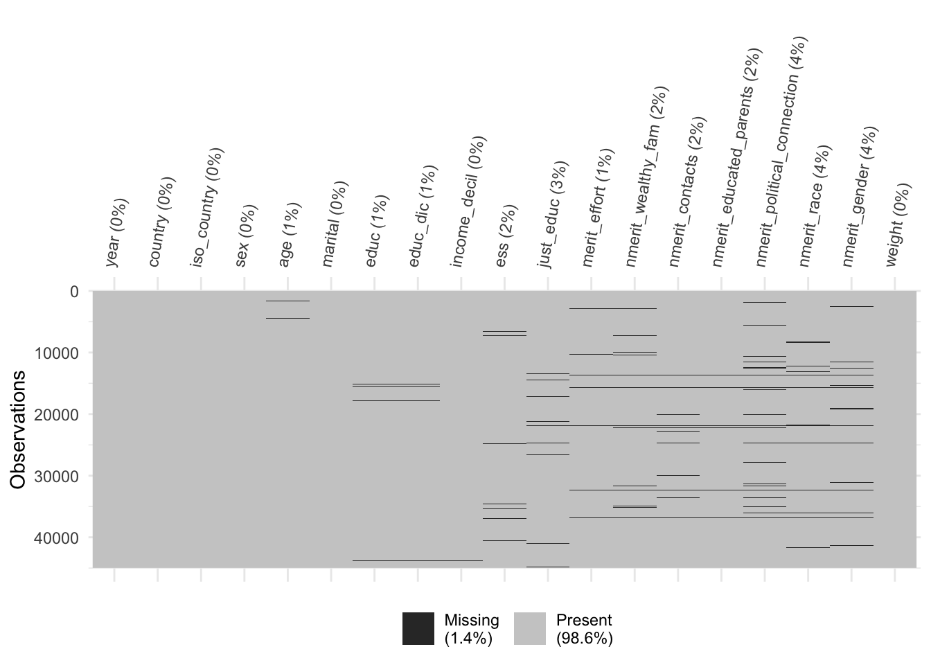
6.4 Save
save(db_proc19, file = here("input/data/proc/db_proc19.RData"))7 Final data
7.1 Merge ISSP
dfs_no_labels <- map(list(db_proc99, db_proc09, db_proc19), remove_all_labels)

names(dfs_no_labels) <- c("db_proc99", "db_proc09", "db_proc19")
list2env(dfs_no_labels, envir = .GlobalEnv)
<environment: R_GlobalEnv>db_proc <- bind_rows(
`1999` = db_proc99,
`2009` = db_proc09,
`2019` = db_proc19,
.id = "source_year"
) %>%
select(-source_year)
db_proc <- tibble::rowid_to_column(db_proc, "id_subject")
head(db_proc) id_subject year country iso_country sex age marital
1 1 1999 Australia AUS Male 58 Married
2 2 1999 Australia AUS Male 45 Married
3 3 1999 Australia AUS Male 66 Married
4 4 1999 Australia AUS Male 20 Not married
5 5 1999 Australia AUS Male 41 Married
6 6 1999 Australia AUS Male 83 Not married
educ educ_dic income_decil ess just_educ
1 Incomplete secondary Less than universitary 4 7 2
2 Incomplete secondary Less than universitary 6 5 3
3 Incomplete secondary Less than universitary 0 4 3
4 Complete secondary Less than universitary NA 2 4
5 Incomplete secondary Less than universitary 4 9 3
6 Incomplete secondary Less than universitary 0 2 2
merit_effort merit_talent nmerit_wealthy_fam nmerit_contacts weight
1 3 2 3 3 1
2 4 3 4 4 1
3 4 4 2 3 1
4 5 5 2 3 1
5 2 2 3 4 1
6 3 2 4 4 1
merit_ambition nmerit_educated_parents nmerit_political_connection
1 NA NA NA
2 NA NA NA
3 NA NA NA
4 NA NA NA
5 NA NA NA
6 NA NA NA
nmerit_race nmerit_gender
1 NA NA
2 NA NA
3 NA NA
4 NA NA
5 NA NA
6 NA NA7.2 Main variables per country and wave
| country_wave | just_educ | merit_effort | merit_talent | merit_ambition | nmerit_wealthy_fam | nmerit_contacts | nmerit_educated_parents | nmerit_political_connection | nmerit_race | nmerit_gender |
|---|---|---|---|---|---|---|---|---|---|---|
| ARG_2009 | 3.80 | 0.44 | 100.00 | 1.41 | 2.03 | 1.94 | 2.12 | 3.27 | 1.85 | 2.65 |
| AUS_1999 | 3.29 | 2.39 | 2.57 | 100.00 | 3.41 | 3.29 | 100.00 | 100.00 | 100.00 | 100.00 |
| AUS_2009 | 3.21 | 1.97 | 100.00 | 1.84 | 3.02 | 1.77 | 2.10 | 6.62 | 4.72 | 5.38 |
| AUS_2019 | 2.90 | 2.15 | 100.00 | 100.00 | 3.56 | 2.90 | 2.15 | 5.34 | 4.31 | 6.27 |
| AUT_1999 | 2.95 | 7.87 | 6.99 | 100.00 | 1.57 | 1.18 | 100.00 | 100.00 | 100.00 | 100.00 |
| AUT_2009 | 1.18 | 0.10 | 100.00 | 0.39 | 1.08 | 0.98 | 0.98 | 2.75 | 4.71 | 2.75 |
| AUT_2019 | 1.19 | 0.08 | 100.00 | 100.00 | 0.16 | 0.32 | 0.08 | 0.95 | 0.87 | 0.71 |
| BEL_2009 | 2.24 | 1.08 | 100.00 | 2.87 | 3.41 | 1.17 | 1.35 | 5.38 | 4.30 | 7.17 |
| BGR_1999 | 5.17 | 3.27 | 3.99 | 100.00 | 2.00 | 2.63 | 100.00 | 100.00 | 100.00 | 100.00 |
| BGR_2009 | 8.30 | 3.60 | 100.00 | 3.80 | 4.40 | 5.50 | 5.10 | 11.50 | 14.50 | 10.50 |
| BGR_2019 | 2.35 | 0.96 | 100.00 | 100.00 | 2.09 | 1.39 | 1.39 | 2.69 | 3.65 | 2.69 |
| CAN_1999 | 1.75 | 1.64 | 4.31 | 100.00 | 1.64 | 0.41 | 100.00 | 100.00 | 100.00 | 100.00 |
| CHE_2009 | 0.65 | 0.08 | 100.00 | 0.16 | 0.81 | 1.14 | 0.73 | 2.20 | 1.06 | 1.06 |
| CHE_2019 | 1.38 | 1.15 | 100.00 | 100.00 | 1.64 | 1.38 | 1.51 | 2.63 | 3.58 | 2.14 |
| CHL_1999 | 4.19 | 2.53 | 3.06 | 100.00 | 2.33 | 2.53 | 100.00 | 100.00 | 100.00 | 100.00 |
| CHL_2009 | 2.72 | 1.06 | 100.00 | 1.26 | 0.66 | 1.99 | 0.86 | 3.26 | 2.59 | 1.46 |
| CHL_2019 | 3.06 | 0.66 | 100.00 | 100.00 | 1.24 | 1.24 | 1.24 | 2.55 | 2.04 | 2.62 |
| CHN_2009 | 4.88 | 0.47 | 100.00 | 1.30 | 0.93 | 0.80 | 0.56 | 1.99 | 2.23 | 3.75 |
| CYP_1999 | 0.40 | 1.30 | 1.40 | 100.00 | 0.00 | 0.00 | 100.00 | 100.00 | 100.00 | 100.00 |
| CYP_2009 | 5.60 | 0.00 | 100.00 | 0.20 | 1.10 | 1.40 | 0.90 | 2.60 | 3.40 | 2.00 |
| CZE_1999 | 2.07 | 3.16 | 4.58 | 100.00 | 2.24 | 2.29 | 100.00 | 100.00 | 100.00 | 100.00 |
| CZE_2009 | 1.66 | 0.91 | 100.00 | 0.83 | 0.66 | 1.08 | 1.24 | 2.49 | 1.83 | 1.49 |
| CZE_2019 | 1.87 | 0.36 | 100.00 | 100.00 | 0.57 | 0.68 | 0.52 | 1.66 | 2.08 | 1.61 |
| DEU_1999 | 2.79 | 7.12 | 4.82 | 100.00 | 3.14 | 2.65 | 100.00 | 100.00 | 100.00 | 100.00 |
| DEU_2009 | 2.37 | 1.86 | 100.00 | 1.36 | 2.94 | 2.15 | 2.29 | 4.80 | 4.44 | 4.73 |
| DEU_2019 | 1.43 | 1.81 | 100.00 | 100.00 | 1.96 | 1.28 | 1.28 | 6.42 | 5.43 | 5.81 |
| DNK_2009 | 4.15 | 1.84 | 100.00 | 1.58 | 2.70 | 2.31 | 1.84 | 10.47 | 4.41 | 6.52 |
| DNK_2019 | 2.60 | 1.54 | 100.00 | 100.00 | 1.25 | 1.54 | 1.06 | 8.67 | 3.85 | 4.53 |
| ESP_1999 | 0.74 | 2.64 | 2.64 | 100.00 | 1.98 | 1.40 | 100.00 | 100.00 | 100.00 | 100.00 |
| ESP_2009 | 2.63 | 1.07 | 100.00 | 1.98 | 1.48 | 1.40 | 1.98 | 3.95 | 3.95 | 7.90 |
| EST_2009 | 1.49 | 0.60 | 100.00 | 4.58 | 1.19 | 1.49 | 0.90 | 7.36 | 1.99 | 3.28 |
| FIN_2009 | 3.07 | 2.39 | 100.00 | 2.73 | 3.75 | 3.41 | 3.98 | 7.95 | 11.48 | 5.45 |
| FIN_2019 | 4.14 | 1.55 | 100.00 | 100.00 | 3.93 | 3.62 | 3.42 | 10.77 | 12.32 | 6.83 |
| FRA_1999 | 1.06 | 1.48 | 2.01 | 100.00 | 1.75 | 1.59 | 100.00 | 100.00 | 100.00 | 100.00 |
| FRA_2009 | 1.77 | 3.16 | 100.00 | 1.17 | 3.73 | 2.59 | 1.35 | 5.75 | 7.95 | 7.70 |
| FRA_2019 | 5.94 | 2.19 | 100.00 | 100.00 | 2.75 | 3.32 | 2.25 | 5.19 | 5.26 | 3.63 |
| GBR_1999 | 2.49 | 4.23 | 3.36 | 100.00 | 3.61 | 2.74 | 100.00 | 100.00 | 100.00 | 100.00 |
| GBR_2009 | 3.03 | 1.25 | 100.00 | 1.36 | 3.13 | 1.67 | 1.88 | 4.59 | 7.72 | 7.72 |
| GBR_2019 | 3.19 | 2.38 | 100.00 | 100.00 | 4.58 | 3.25 | 2.61 | 6.15 | 6.44 | 7.71 |
| HRV_2009 | 2.66 | 1.58 | 100.00 | 0.83 | 1.58 | 1.42 | 1.58 | 4.00 | 4.66 | 4.66 |
| HRV_2019 | 1.00 | 0.20 | 100.00 | 100.00 | 0.40 | 0.40 | 0.30 | 2.30 | 2.60 | 2.70 |
| HUN_1999 | 1.32 | 1.32 | 2.32 | 100.00 | 0.99 | 2.90 | 100.00 | 100.00 | 100.00 | 100.00 |
| HUN_2009 | 1.29 | 0.69 | 100.00 | 0.30 | 0.30 | 0.20 | 0.50 | 2.38 | 2.08 | 0.99 |
| IRL_1999 | 3.01 | 6.02 | 5.42 | 100.00 | 2.77 | 2.77 | 100.00 | 100.00 | 100.00 | 100.00 |
| ISL_2009 | 0.53 | 0.21 | 100.00 | 0.42 | 0.74 | 0.63 | 0.42 | 2.11 | 2.43 | 3.91 |
| ISL_2019 | 1.22 | 0.24 | 100.00 | 100.00 | 0.49 | 0.49 | 0.49 | 3.26 | 3.10 | 4.56 |
| ISR_1999 | 0.83 | 0.50 | 0.75 | 100.00 | 0.17 | 0.08 | 100.00 | 100.00 | 100.00 | 100.00 |
| ISR_2009 | 2.26 | 1.17 | 100.00 | 1.17 | 0.42 | 0.75 | 0.84 | 1.76 | 1.68 | 1.76 |
| ISR_2019 | 0.67 | 0.17 | 100.00 | 100.00 | 0.25 | 0.50 | 0.25 | 1.50 | 1.67 | 2.00 |
| ITA_2009 | 1.75 | 5.07 | 100.00 | 5.07 | 6.00 | 5.07 | 5.81 | 10.89 | 9.78 | 8.49 |
| ITA_2019 | 2.55 | 1.15 | 100.00 | 100.00 | 1.32 | 1.15 | 1.32 | 3.46 | 3.46 | 2.80 |
| JPN_1999 | 4.83 | 2.42 | 2.72 | 100.00 | 5.66 | 7.09 | 100.00 | 100.00 | 100.00 | 100.00 |
| JPN_2009 | 8.02 | 2.78 | 100.00 | 6.02 | 4.48 | 8.80 | 4.55 | 13.19 | 13.12 | 8.41 |
| JPN_2019 | 8.01 | 4.55 | 100.00 | 100.00 | 6.45 | 11.13 | 6.31 | 12.90 | 14.87 | 11.61 |
| KOR_2009 | 1.00 | 0.13 | 100.00 | 0.25 | 0.25 | 0.25 | 0.13 | 1.25 | 1.19 | 0.50 |
| LTU_2009 | 3.71 | 2.05 | 100.00 | 3.42 | 2.15 | 2.74 | 1.47 | 7.43 | 4.40 | 8.50 |
| LTU_2019 | 4.76 | 1.52 | 100.00 | 100.00 | 2.00 | 2.29 | 1.33 | 5.62 | 3.43 | 3.52 |
| LVA_1999 | 2.45 | 1.73 | 2.27 | 100.00 | 1.36 | 0.91 | 100.00 | 100.00 | 100.00 | 100.00 |
| LVA_2009 | 0.47 | 0.09 | 100.00 | 1.40 | 0.47 | 0.28 | 0.37 | 2.15 | 2.34 | 3.74 |
| NOR_1999 | 2.68 | 2.44 | 3.39 | 100.00 | 1.74 | 1.42 | 100.00 | 100.00 | 100.00 | 100.00 |
| NOR_2009 | 6.82 | 1.85 | 100.00 | 1.85 | 2.33 | 3.93 | 1.93 | 6.98 | 8.35 | 6.18 |
| NOR_2019 | 1.89 | 2.95 | 100.00 | 100.00 | 4.08 | 2.87 | 5.06 | 7.63 | 8.31 | 5.82 |
| NZL_1999 | 3.25 | 2.53 | 2.08 | 100.00 | 2.62 | 1.81 | 100.00 | 100.00 | 100.00 | 100.00 |
| NZL_2009 | 3.32 | 0.53 | 100.00 | 1.39 | 3.42 | 1.71 | 1.71 | 2.89 | 2.78 | 3.64 |
| NZL_2019 | 2.81 | 1.65 | 100.00 | 100.00 | 2.48 | 1.57 | 1.90 | 3.72 | 2.89 | 4.63 |
| PHL_1999 | 0.83 | 0.17 | 0.33 | 100.00 | 0.33 | 0.50 | 100.00 | 100.00 | 100.00 | 100.00 |
| PHL_2009 | 1.17 | 0.00 | 100.00 | 0.00 | 0.08 | 0.33 | 0.42 | 1.08 | 1.33 | 0.83 |
| PHL_2019 | 0.71 | 0.21 | 100.00 | 100.00 | 0.49 | 0.47 | 0.26 | 0.94 | 0.66 | 0.80 |
| POL_1999 | 8.19 | 10.66 | 13.39 | 100.00 | 6.26 | 4.41 | 100.00 | 100.00 | 100.00 | 100.00 |
| POL_2009 | 2.93 | 0.63 | 100.00 | 1.11 | 1.66 | 2.30 | 1.11 | 9.98 | 7.60 | 8.87 |
| PRT_1999 | 0.61 | 0.44 | 1.92 | 100.00 | 1.22 | 1.05 | 100.00 | 100.00 | 100.00 | 100.00 |
| PRT_2009 | 2.00 | 0.10 | 100.00 | 0.30 | 0.50 | 0.40 | 0.20 | 4.00 | 2.90 | 1.10 |
| RUS_1999 | 4.69 | 3.11 | 5.69 | 100.00 | 4.93 | 3.75 | 100.00 | 100.00 | 100.00 | 100.00 |
| RUS_2009 | 7.11 | 1.25 | 100.00 | 6.49 | 3.87 | 2.43 | 2.56 | 10.11 | 7.24 | 6.67 |
| RUS_2019 | 2.19 | 0.63 | 100.00 | 100.00 | 3.38 | 0.94 | 1.75 | 6.45 | 2.82 | 2.76 |
| SUR_2019 | 14.59 | 3.70 | 100.00 | 100.00 | 6.39 | 5.89 | 4.60 | 6.69 | 7.39 | 8.59 |
| SVK_1999 | 1.29 | 1.02 | 1.85 | 100.00 | 0.46 | 0.83 | 100.00 | 100.00 | 100.00 | 100.00 |
| SVK_2009 | 2.07 | 0.60 | 100.00 | 0.86 | 0.78 | 0.95 | 0.69 | 2.85 | 1.21 | 1.38 |
| SVN_1999 | 0.89 | 2.98 | 4.77 | 100.00 | 2.19 | 1.29 | 100.00 | 100.00 | 100.00 | 100.00 |
| SVN_2009 | 3.10 | 0.85 | 100.00 | 1.97 | 1.31 | 1.03 | 1.31 | 3.66 | 5.73 | 2.91 |
| SVN_2019 | 1.29 | 0.52 | 100.00 | 100.00 | 1.12 | 0.60 | 0.60 | 4.12 | 3.44 | 2.15 |
| SWE_1999 | 1.65 | 5.22 | 6.00 | 100.00 | 5.04 | 2.70 | 100.00 | 100.00 | 100.00 | 100.00 |
| SWE_2009 | 2.90 | 2.81 | 100.00 | 2.46 | 4.05 | 3.17 | 3.08 | 9.23 | 9.85 | 7.30 |
| SWE_2019 | 2.38 | 2.02 | 100.00 | 100.00 | 3.73 | 2.93 | 3.06 | 10.33 | 8.44 | 5.56 |
| THA_2019 | 4.96 | 3.13 | 100.00 | 100.00 | 2.09 | 4.76 | 1.83 | 5.74 | 5.22 | 5.09 |
| TUR_2009 | 5.93 | 0.76 | 100.00 | 1.53 | 1.59 | 1.21 | 1.34 | 4.08 | 7.52 | 4.33 |
| TWN_2009 | 0.74 | 0.10 | 100.00 | 0.64 | 0.64 | 0.25 | 0.49 | 1.43 | 1.23 | 0.99 |
| TWN_2019 | 0.83 | 0.05 | 100.00 | 100.00 | 1.04 | 0.93 | 0.83 | 1.66 | 0.83 | 0.36 |
| UKR_2009 | 7.16 | 3.58 | 100.00 | 7.85 | 4.22 | 4.62 | 2.88 | 14.76 | 6.51 | 7.16 |
| USA_1999 | 5.97 | 6.21 | 5.82 | 100.00 | 7.55 | 5.90 | 100.00 | 100.00 | 100.00 | 100.00 |
| USA_2009 | 3.54 | 0.38 | 100.00 | 1.33 | 3.29 | 0.82 | 1.27 | 4.05 | 3.73 | 4.49 |
| USA_2019 | 4.48 | 1.35 | 100.00 | 100.00 | 3.62 | 1.94 | 1.94 | 4.37 | 4.27 | 4.54 |
| VEN_2009 | 0.83 | 0.41 | 100.00 | 0.52 | 0.72 | 1.24 | 1.03 | 3.61 | 2.68 | 2.37 |
| VEN_2019 | 2.77 | 1.61 | 100.00 | 100.00 | 1.52 | 2.23 | 1.07 | 2.14 | 8.31 | 7.51 |
| ZAF_2009 | 3.09 | 0.91 | 100.00 | 1.00 | 1.42 | 1.15 | 1.00 | 3.72 | 1.39 | 1.36 |
| ZAF_2019 | 2.97 | 0.40 | 100.00 | 100.00 | 0.66 | 0.40 | 0.55 | 1.72 | 1.03 | 1.32 |