
| Components | Dimensions | Item (English) | Item original (Spanish) |
|---|---|---|---|
| Perception | Meritocratic | In Chile people are rewarded for their efforts | En Chile las personas son recompensadas por sus esfuerzos |
| In Chile people are rewarded for their intelligence and ability | En Chile las personas son recompensadas por su inteligencia y habilidad | ||
| Non meritocratic | In Chile those with wealthy parents do much better in life | En Chile a quienes tienen padres ricos les va mucho mejor en la vida | |
| In Chile those with good contacts do much better in life | En Chile a quienes tienen buenos contactos les va mejor en la vida | ||
| Preference | Meritocratic | Those who work harder should reap greater rewards than those who work less hard | Quienes más se esfuerzan deberían obtener mayores recompensas que quienes se esfuerzan menos |
| Those with more talent should reap greater rewards than those with less talent | Quienes poseen más talento deberían obtener mayores recompensas que quienes poseen menos talento | ||
| Non meritocratic | It is good that those who have rich parents do better in life | Está bien que quienes tengan padres ricos les vaya mejor en la vida | |
| It is good that those who have good contacts do better in life | Está bien que quienes tengan buenos contactos les vaya mejor en la vida |
1 Aim
This study applies latent class analysis (LCA) to a multidimensional scale of meritocratic beliefs developed by Castillo et al. (2023) to identify distinct latent profiles of how individuals combine meritocratic and non-meritocratic beliefs.
Rather than focusing on validating the measurement model, the analysis seeks to uncover patterns of response configurations across items, thereby identifying underlying typologies of meritocratic orientations.
The dataset used is db_proc.RData generated in the prod_prep.R script.
2 Data
- Dataset: EDUMERCO (2025)
- Mode: Online survey (CAWI)
- Population: Adults in the Metropolitan Region of Chile
- Sampling: Non-probability quota-based design
- Quotas based on age, gender, education, and socioeconomic status
- Sample size: N = 3,470
- Analytical sample: N = 2,740
3 Measures
3.1 Meritocracy scale
We use a multidimensional scale that distinguishes between (Table 1):
- Perceptions and preferences
- Meritocratic and non-meritocratic principles
This results in four dimensions:
- Perceived meritocracy: beliefs about whether effort and ability are rewarded
- Perceived non-meritocracy: beliefs about the role of connections and family wealth
- Preference for meritocracy: normative support for rewarding effort and talent
- Preference for non-meritocracy: normative acceptance of advantages linked to privilege
Each dimension is measured with two items, for a total of eight items. Responses are recorded on a four-point Likert scale ranging from strongly disagree (1) to strongly agree (4).
4 Method
4.1 Latent class analysis
Latent class analysis (LCA) is a statistical method that models associations among observed variables by assuming that an unobserved categorical latent variable explains their underlying structure. This latent variable represents discrete subgroups within the population, where individuals in the same class share similar response patterns.
LCA is especially appropriate for categorical and ordinal indicators, such as Likert-scale items.
4.1.1 Analytical purpose
LCA can serve both exploratory and confirmatory purposes.
- As an exploratory technique, it identifies latent typologies of belief configurations.
- As a confirmatory technique, it allows researchers to test hypotheses about heterogeneity in the population.
Substantively, LCA enables the derivation of empirically grounded ideal types of meritocratic orientations.
4.1.2 Key assumptions
- Each individual belongs to one latent class.
- Individuals within the same class share similar response probabilities.
- Observed indicators are conditionally independent once class membership is taken into account (local independence).
4.1.3 Model parameters
The model estimates two main sets of parameters:
Class probabilities
These indicate the probability of belonging to each latent class and reflect the relative size of each group in the population.Conditional response probabilities
These indicate the probability of endorsing a particular response category, given membership in a latent class. These parameters are used to interpret and label the classes.
4.2 Interpretation
Latent classes are defined by distinct response profiles across the eight items. These profiles capture different combinations of:
- meritocratic and non-meritocratic beliefs
- perceptions and normative preferences
This allows us to identify complex belief systems in which individuals may, for example, endorse meritocratic ideals while simultaneously recognizing, or even accepting, non-meritocratic advantages.
4.3 Model estimation and fit
Models are estimated iteratively by increasing the number of classes.
Model selection is based primarily on standard fit criteria, especially:
- Bayesian Information Criterion (BIC)
- Akaike Information Criterion (AIC)
Lower values indicate a better fit, while also balancing model complexity and parsimony.
4.4 Contribution
This strategy shifts the analysis from a variable-centered approach to a person-centered one. In doing so, it allows us to:
- capture heterogeneity in meritocratic belief systems
- identify meaningful subgroups of respondents
- examine how meritocratic and non-meritocratic beliefs coexist within individuals
5 Libraries
6 Data
Show the code
load(here("input/data/proc/db_proc.RData"))

glimpse(db)
Rows: 3,470
Columns: 25
$ id <int> 1, 2, 3, 4, 5, 6, 7, 8, 9, 10, 11, 12, 13, 14, 15,…
$ just_pension <fct> Agree, Strongly desagree, Strongly desagree, Stron…
$ perc_effort <fct> Desagree, Strongly desagree, Strongly desagree, De…
$ perc_talent <fct> Desagree, Desagree, Desagree, Desagree, Agree, Des…
$ perc_rich_parents <fct> Agree, Strongly agree, Strongly agree, Strongly ag…
$ perc_contact <fct> Strongly agree, Agree, Strongly agree, Strongly ag…
$ perc_effort_d <fct> Low, Low, Low, Low, High, Low, Low, NA, High, Low,…
$ perc_talent_d <fct> Low, Low, Low, Low, High, Low, Low, NA, High, Low,…
$ perc_rich_parents_d <fct> High, High, High, High, High, High, Low, High, Hig…
$ perc_contact_d <fct> High, High, High, High, High, High, High, High, Hi…
$ pref_effort <fct> Strongly agree, Strongly agree, Strongly agree, St…
$ pref_talent <fct> Strongly agree, Agree, Agree, Desagree, Strongly a…
$ pref_rich_parents <fct> Agree, Strongly agree, Desagree, Strongly agree, A…
$ pref_contact <fct> Desagree, Strongly agree, Desagree, Strongly agree…
$ pref_effort_d <fct> High, High, High, High, High, High, High, NA, High…
$ pref_talent_d <fct> High, High, High, Low, High, High, NA, NA, High, H…
$ pref_rich_parents_d <fct> High, High, Low, High, High, Low, Low, NA, Low, Lo…
$ pref_contact_d <fct> Low, High, Low, High, Low, Low, Low, NA, Low, Low,…
$ age <int> 72, 67, 65, 59, 57, 69, 65, 68, 65, 65, 58, 56, 35…
$ sex <fct> 1, 2, 1, 2, 2, 1, 2, 2, 1, 2, 2, 2, 2, 1, 1, 1, 2,…
$ educ <int> 6, 4, 8, 5, 6, 8, 8, 6, 6, 6, 4, 9, 4, 5, 8, 8, 6,…
$ income <fct> De $890.001 a $1.100.000 mensuales liquidos, De $3…
$ pol <fct> Right, Does not identify, Left, Does not identify,…
$ just_educ <fct> Desagree, Strongly desagree, Strongly desagree, St…
$ just_healthcare <fct> Desagree, Strongly desagree, Strongly desagree, St…Show the code
db <- db %>%
  mutate(
    income_4 = case_when(
      income %in% c(
        "Menos de $280.000 mensuales liquidos",
        "De $280.001 a $380.000 mensuales liquidos",
        "De $380.001 a $470.000 mensuales liquidos"
      ) ~ "Low",

      income %in% c(
        "De $470.001 a $610.000 mensuales liquidos",
        "De $610.001 a $730.000 mensuales liquidos"
      ) ~ "Middle-low",

      income %in% c(
        "De $730.001 a $890.000 mensuales liquidos",
        "De $890.001 a $1.100.000 mensuales liquidos"
      ) ~ "Middle-high",

      income %in% c(
        "De $1.100.001 a $2.700.000 mensuales liquidos",
        "De $2.700.001 a $4.100.000 mensuales liquidos",
        "Mas de $4.100.001 mensuales liquidos"
      ) ~ "High",

      TRUE ~ NA_character_
    ),
    income_4 = factor(income_4, levels = c("Low", "Middle-low", "Middle-high", "High"))
  )


db$income_4 <- sjlabelled::set_label(db$income_4, "Income")

db$age <- sjlabelled::set_label(db$age, "Age")

db$sex <- if_else(db$sex == 1, "Male", "Female")

db$sex <- factor(db$sex, levels = c("Male", "Female"))

db$sex <- sjlabelled::set_label(db$sex, "Sex")

db$educ <- sjlabelled::set_label(db$educ, "Educational level")


db$pol <- sjlabelled::set_label(db$pol, "Political identification")
7 Analysis
7.1 Descriptives
Show the code
vars_m <- c("perc_effort",
            "perc_talent",
            "perc_rich_parents",
            "perc_contact",
            "pref_effort",
            "pref_talent",
            "pref_rich_parents",
            "pref_contact")

t1 <- db %>%
   dplyr::select(all_of(vars_m), age, sex, educ, income_4, pol)


df<-dfSummary(t1,
               plain.ascii = FALSE,
               style = "multiline",
               tmp.img.dir = "/tmp",
               graph.magnif = 0.75,
               headings = F,  # encabezado
               varnumbers = F, # num variable
               labels.col = T, # etiquetas
               na.col = T,    # missing
               graph.col = T, # plot
               valid.col = T, # n valido
               col.widths = c(20,10,10,10,10,10))

df$Variable <- NULL # delete variable column

print(df, method="render")| Label | Stats / Values | Freqs (% of Valid) | Graph | Valid | Missing | ||||||||||||||||||||||||||||||||||||||||||||||||||||||||||
|---|---|---|---|---|---|---|---|---|---|---|---|---|---|---|---|---|---|---|---|---|---|---|---|---|---|---|---|---|---|---|---|---|---|---|---|---|---|---|---|---|---|---|---|---|---|---|---|---|---|---|---|---|---|---|---|---|---|---|---|---|---|---|---|
| In Chile people are rewarded for their efforts |
|
|
 |
3312 (95.4%) | 158 (4.6%) | ||||||||||||||||||||||||||||||||||||||||||||||||||||||||||
| In Chile people are rewarded for their intelligence and ability |
|
|
 |
3311 (95.4%) | 159 (4.6%) | ||||||||||||||||||||||||||||||||||||||||||||||||||||||||||
| In Chile those with wealthy parents do much better in life |
|
|
 |
3356 (96.7%) | 114 (3.3%) | ||||||||||||||||||||||||||||||||||||||||||||||||||||||||||
| In Chile those with good contacts do much better in life |
|
|
 |
3389 (97.7%) | 81 (2.3%) | ||||||||||||||||||||||||||||||||||||||||||||||||||||||||||
| Those who work harder should reap greater rewards than those who work less hard |
|
|
 |
3341 (96.3%) | 129 (3.7%) | ||||||||||||||||||||||||||||||||||||||||||||||||||||||||||
| Those with more talent should reap greater rewards than those with less talent |
|
|
 |
3207 (92.4%) | 263 (7.6%) | ||||||||||||||||||||||||||||||||||||||||||||||||||||||||||
| It is good that those who have rich parents do better in life |
|
|
 |
3092 (89.1%) | 378 (10.9%) | ||||||||||||||||||||||||||||||||||||||||||||||||||||||||||
| It is good that those who have good contacts do better in life |
|
|
 |
3179 (91.6%) | 291 (8.4%) | ||||||||||||||||||||||||||||||||||||||||||||||||||||||||||
| Age |
|
70 distinct values |  |
3470 (100.0%) | 0 (0.0%) | ||||||||||||||||||||||||||||||||||||||||||||||||||||||||||
| Sex |
|
|
 |
3446 (99.3%) | 24 (0.7%) | ||||||||||||||||||||||||||||||||||||||||||||||||||||||||||
| Educational level |
|
|
 |
3470 (100.0%) | 0 (0.0%) | ||||||||||||||||||||||||||||||||||||||||||||||||||||||||||
| Income |
|
|
 |
3470 (100.0%) | 0 (0.0%) | ||||||||||||||||||||||||||||||||||||||||||||||||||||||||||
| Political identification |
|
|
 |
3321 (95.7%) | 149 (4.3%) |
Generated by summarytools 1.1.5 (R version 4.5.2)
2026-04-01
Show the code
db <- db %>%
  mutate(
    across(
      .cols = all_of(vars_m),
      .fns = ~as.numeric(.)
    ))

labels1 <- c("Strongly desagree" = 1,
             "Desagree" = 2,
             "Agree" = 3,
             "Strongly agree" = 4)
db <- db %>%
  mutate(
    across(
      .cols = all_of(vars_m),
      .fns = ~  sjlabelled::set_labels(., labels = labels1)
    )
  )


df <- db %>%
  dplyr::select(all_of(vars_m)) %>%
  drop_na()

theme_set(theme_ggdist())
colors <- RColorBrewer::brewer.pal(n = 4, name = "RdBu")


a <- df %>%
  dplyr::select(perc_effort,
                perc_talent,
                perc_rich_parents,
                perc_contact) %>%
  sjPlot::plot_likert(geom.colors = colors,
                      title = c("a. Perceptions"),
                      geom.size = 0.8,
                      axis.labels = c("Effort", "Talent", "Rich parents", "Contacts"),
                      catcount = 4,
                      values  =  "sum.outside",
                      reverse.colors = F,
                      reverse.scale = T,
                      show.n = FALSE,
                      show.prc.sign = T
  ) +
  ggplot2::theme(legend.position = "none")

b <- df %>%
  dplyr::select(pref_effort,
                pref_talent,
                pref_rich_parents,
                pref_contact) %>%
  sjPlot::plot_likert(geom.colors = colors,
                      title = c("b. Preferences"),
                      geom.size = 0.8,
                      axis.labels = c("Effort", "Talent", "Rich parents", "Contacts"),
                      catcount = 4,
                      values  =  "sum.outside",
                      reverse.colors = F,
                      reverse.scale = T,
                      show.n = FALSE,
                      show.prc.sign = T
  ) +
  ggplot2::theme(legend.position = "bottom")

likerplot <- a / b + plot_annotation(caption = paste0("Source: own elaboration based on Survey EDUMERCO"," (n = ",dim(df)[1],")"
))

likerplot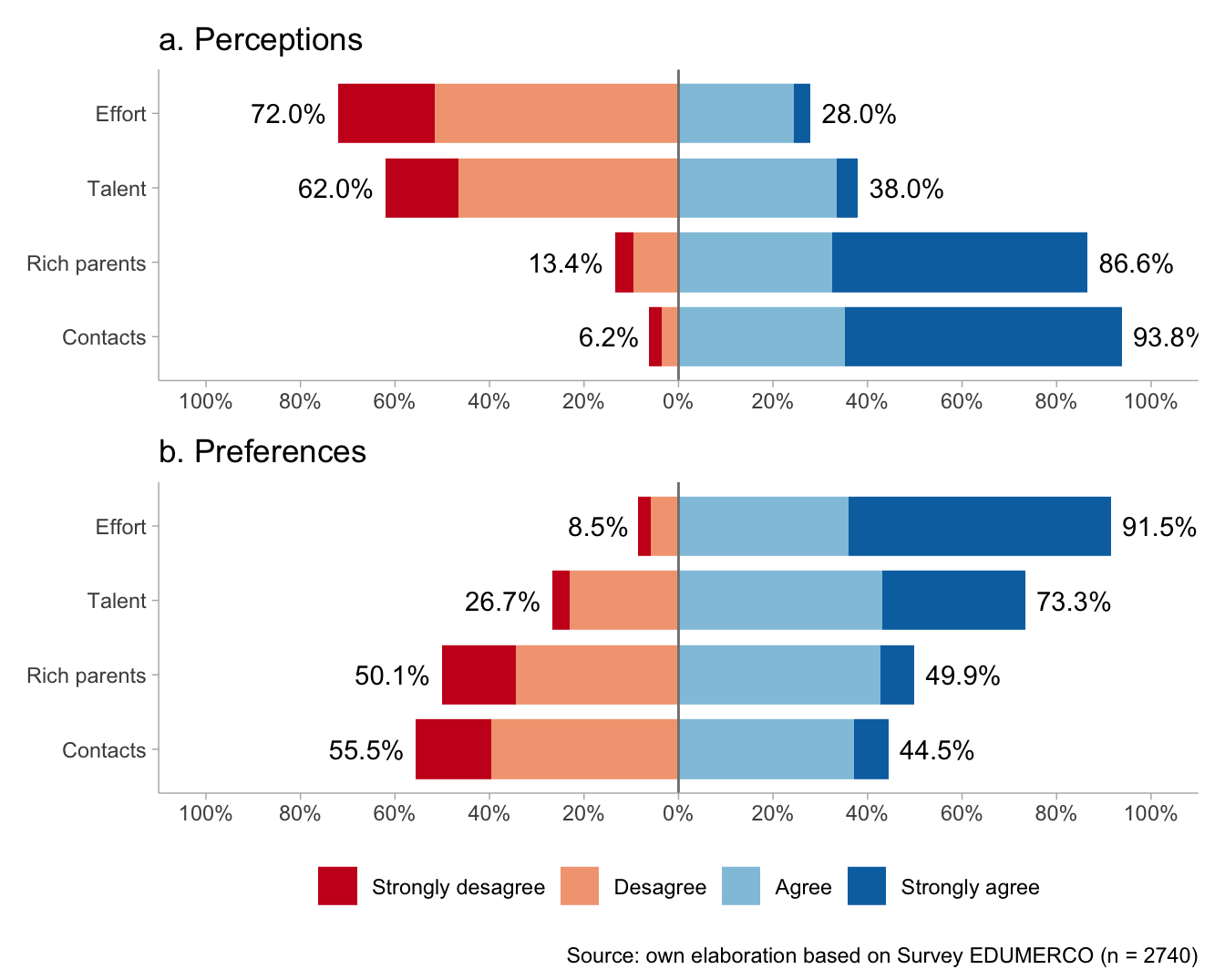
Show the code
M <- df %>%
  psych::polychoric()

diag(M$rho) <- NA

rownames(M$rho) <- c("A. Perception Effort",
                     "B. Perception Talent",
                     "C. Perception Rich parents",
                     "D. Perception Contacts",
                     "E. Preference Effort",
                     "F. Preference Talent",
                     "G. Preference Rich parents",
                     "H. Preference Contacts")

#set Column names of the matrix
colnames(M$rho) <-c("(A)", "(B)","(C)","(D)","(E)","(F)","(G)",
                    "(H)")

testp <- cor.mtest(M$rho, conf.level = 0.95)

#Plot the matrix using corrplot
corrplot::corrplot(M$rho,
                   method = "color",
                   addCoef.col = "black",
                   type = "upper",
                   tl.col = "black",
                   col = colorRampPalette(c("#E16462", "white", "#0D0887"))(12),
                   bg = "white",
na.label = "-") 
7.2 Latent class analysis with dichotomized items
We estimated latent class models with one to five classes. Model fit improved monotonically as the number of classes increased, as indicated by decreasing AIC and BIC values and statistically significant likelihood-ratio tests at each step (Table 3).
Show the code
# ---- build table (no list-cols) -----------------------------------------

N_used <- nrow(db_lca)

m_patterns <- n_patterns_from_data(db_lca)  # scalar

# Robust extractors (avoid list-columns)
get_K <- function(fit) as.integer(ncol(fit$posterior))  # classes = cols of posterior
get_ll  <- function(fit) as.numeric(fit$llik)
get_aic <- function(fit) as.numeric(fit$aic)
get_bic <- function(fit) as.numeric(fit$bic)
get_npar <- function(fit) {
  if (!is.null(fit$npar)) return(as.numeric(fit$npar))
  # fallback: compute from probs
  K <- get_K(fit)
  Rj <- vapply(fit$probs, function(m) ncol(m), integer(1))
  as.numeric(sum(K * (Rj - 1)) + (K - 1))
}

# Table of fit indices
fit_tbl <- tibble(
  K     = map_int(fits, get_K),
  N     = nrow(db_lca),
  logLik= map_dbl(fits, get_ll),
  npar  = map_dbl(fits, get_npar),
  AIC   = map_dbl(fits, get_aic),
  BIC   = map_dbl(fits, get_bic)
) %>%
  arrange(K) %>%
  mutate(
    # Differences relative to preceding (K-1) model
    dAIC = AIC - lag(AIC),
    dBIC = BIC - lag(BIC),

    # Likelihood-ratio test (K vs K-1)
    # Test statistic: 2*(LL_K - LL_{K-1}) ~ Chi-square with df = npar_K - npar_{K-1}
    # Note: in LCA, models are not strictly nested in the regular sense;
    # this LRT is widely used as a heuristic, but interpret with caution.
    LRT = 2 * (logLik - lag(logLik)),
    df_LRT = npar - lag(npar),
    p_LRT = ifelse(!is.na(LRT) & df_LRT > 0, pchisq(LRT, df = df_LRT, lower.tail = FALSE), NA_real_)
  )


fit_tbl_report <- fit_tbl %>%
  transmute(
    K, N,
    logLik = round(logLik, 1),
    npar = npar,
    AIC = round(AIC, 1),
    dAIC = round(dAIC, 1),
    BIC = round(BIC, 1),
    dBIC = round(dBIC, 1),
    LRT = round(LRT, 1),
    df_LRT = df_LRT,
    p_LRT = signif(p_LRT, 3)
  )

fit_tbl_report %>%
 kableExtra::kable(format = "html",
                    align = "c",
                    booktabs = T,
                    escape = F,
                    caption = NULL) %>%
  kableExtra::kable_styling(full_width = T,
                            latex_options = "hold_position",
                            bootstrap_options=c("striped", "bordered", "condensed"),
                            font_size = 23) %>%
  kableExtra::column_spec(c(1,8), width = "3.5cm") %>%
  kableExtra::column_spec(2:7, width = "4cm") %>%
kableExtra::column_spec(4, width = "5cm")| K | N | logLik | npar | AIC | dAIC | BIC | dBIC | LRT | df_LRT | p_LRT |
|---|---|---|---|---|---|---|---|---|---|---|
| 1 | 2740 | -11331.7 | 8 | 22679.5 | 22726.8 | |||||
| 2 | 2740 | -10793.8 | 17 | 21621.6 | -1057.8 | 21722.2 | -1004.6 | 1075.8 | 9 | 0 |
| 3 | 2740 | -10457.9 | 26 | 20967.8 | -653.9 | 21121.6 | -600.6 | 671.9 | 9 | 0 |
| 4 | 2740 | -10162.8 | 35 | 20395.7 | -572.1 | 20602.7 | -518.9 | 590.1 | 9 | 0 |
| 5 | 2740 | -10080.8 | 44 | 20249.6 | -146.0 | 20509.9 | -92.8 | 164.0 | 9 | 0 |
Show the code
# Visual: AIC/BIC by K (lower is better)
fit_long <- fit_tbl %>%
  dplyr::select(K, AIC, BIC) %>%
  pivot_longer(-K, names_to = "criterion", values_to = "value")

ggplot(fit_long, aes(x = K, y = value, group = criterion)) +
  geom_line() +
  geom_point() +
  facet_wrap(~criterion, scales = "free_y") +
labs(x = "Number of classes (K)", y = "Value") 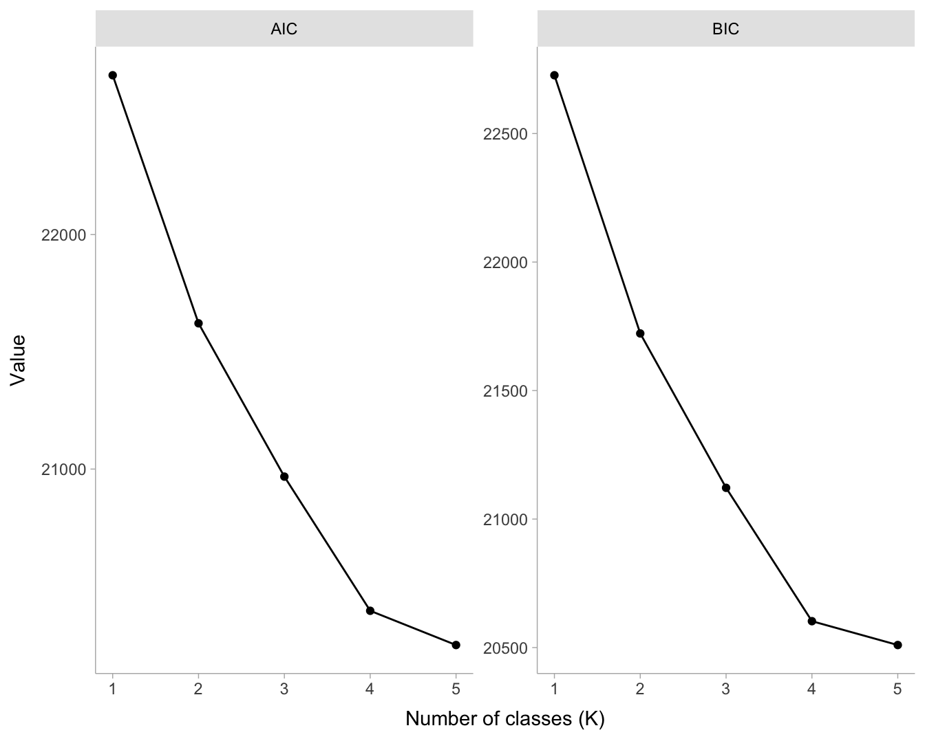
Show the code
# Visual: ΔAIC and ΔBIC (negative = improvement over K-1)
delta_long <- fit_tbl %>%
  dplyr::select(K, dAIC, dBIC) %>%
  pivot_longer(-K, names_to = "delta", values_to = "value")

ggplot(delta_long, aes(x = K, y = value, group = delta)) +
  geom_hline(yintercept = 0) +
  geom_line() +
  geom_point() +
  facet_wrap(~delta, scales = "free_y") +
labs(x = "K", y = "Change vs K-1 (negative = better)") 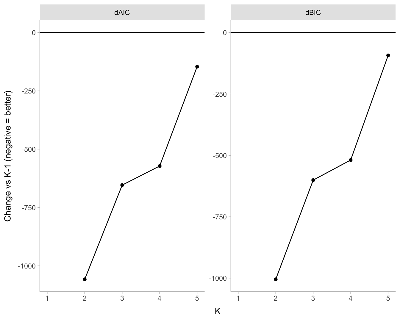
However, the incremental improvement in fit became substantially smaller after the four-class solution. Whereas the transition from one to four classes yielded large reductions in AIC and BIC, the five-class model provided only a modest additional improvement (AIC = 20,249.6; BIC = 20,509.9) relative to the four-class solution (AIC = 20,395.7; BIC = 20,602.7). Thus, although the five-class model fit the data slightly better in statistical terms, the gain was comparatively limited.
We therefore retained the four-class solution as the final model. This choice was guided by both statistical and substantive criteria: the four-class model achieved a strong balance between goodness of fit, parsimony, and interpretability, whereas the five-class solution did not yield enough additional differentiation to justify the increase in complexity.
7.3 Four latent class model
The Table 4 shows the conditional probabilities of each item associated with a latent class and their respective sizes. The four-class solution suggests that respondents are not primarily differentiated along a simple continuum from “more meritocratic” to “less meritocratic.” Instead, the latent classes are organized by distinct combinations of: (1) perceptions of meritocracy, (2) perceptions of non-meritocratic advantage, and (3) normative preferences regarding whether merit or privilege should determine success. As such, the results reveal heterogeneity not only in empirical diagnoses of how society works, but also in normative evaluations of whether these mechanisms are considered acceptable. This interpretation is consistent with the item-response profiles across classes.
Two broader patterns structure the class solution. First, perceptions of non-meritocratic advantage are high across most classes, particularly regarding the role of wealthy parents and personal connections, suggesting that recognition of privilege is widespread. Second, the main line of differentiation lies in normative preferences toward non-meritocratic advantage. In other words, the classes differ less in whether they perceive privilege and more in whether they consider such privilege legitimate or acceptable.
Show the code
fit4 <- fits[[4]]

# 2) Extract conditional probabilities per item and class
# fit4$probs is a list: each element is K x Rj matrix.
# For dichotomous items: K x 2 (categories = colnames or "1","2")
probs_long <- bind_rows(lapply(names(fit4$probs), function(item) {
  mat <- fit4$probs[[item]]
  df <- as.data.frame(mat)
  df$class <- 1:nrow(mat)
  df$item <- item
  df
})) %>%
  pivot_longer(cols = -c(class, item), names_to = "category", values_to = "prob") %>%
  mutate(
    class = as.integer(class),
    prob = as.numeric(prob)
  )

# If levels are c("0","1") or c("1","2") you'll want the "higher"/"yes" one.
# Here I will assume endorsement is the LAST level (most common after dichotomization).
endorsement_level <- tail(levels(db_lca$a1), 1)

# 4) Build a clean table: P(endorsement | class) for each item
p_endorse <- probs_long %>%
  filter(category == "Pr(2)") %>%
  dplyr::select(item, class, p = prob) %>%
  mutate(item = factor(item, levels = names(fit4$probs)))

# 5) Plot: profile lines (one line per class)
p_endorse <- p_endorse %>%
  mutate(
    variable = case_when(item == "a1" ~ "perc_effort",
                         item == "a2" ~ "perc_talent",
                         item == "a3" ~ "perc_rich_parents",
                         item == "a4" ~ "perc_contacts",
                         item == "a5" ~ "pref_effort",
                         item == "a6" ~ "pref_talent",
                         item == "a7" ~ "pref_rich_parents",
                         item == "a8" ~ "pref_contacts"
                         ),
    variable = factor(variable,
                      levels = c("perc_effort",
                                 "perc_talent",
                                 "perc_rich_parents",
                                 "perc_contacts",
                                 "pref_effort",
                                 "pref_talent",
                                 "pref_rich_parents",
                                 "pref_contacts")))

p_endorse <- p_endorse %>%
  mutate(class = factor(class),
         p = round(p,2))

g_class <- ggplot(p_endorse, aes(x = variable, y = p, group = class, colour = class)) +
  geom_line(linewidth = 0.7) +
  geom_point(size = 2) +
  MetBrewer::scale_color_met_d("VanGogh2") +
  coord_cartesian(ylim = c(0, 1)) +
  labs(x = "Item", y = paste0("P(Y = ", "High", " | class)"), group = "Class", colour = "Class") +
  theme(legend.position = "top",
        text = element_text(size = 14),
        axis.text.x = element_text(angle = 70, vjust = 1, hjust = 1))


library(plotly)

ggplotly(g_class)Show the code
# 7) Report table (wide): items x classes with probabilities
class_prev <- tibble(
  class = 1:length(fit4$P),
  pi = as.numeric(fit4$P)
) %>%
  mutate(pi_pct = 100 * pi)

report_probs <- p_endorse %>%
  mutate(class = paste0("Class_", class)) %>%
  pivot_wider(names_from = class, values_from = p) %>%
  mutate(across(starts_with("Class_"), ~ round(.x, 3)))

prev_lab <- class_prev %>%
  transmute(class = paste0("Class_", class),
            lab = paste0(class, " (", round(pi_pct, 1), "%)"))

report_probs2 <- report_probs
for (i in seq_len(nrow(prev_lab))) {
  old <- prev_lab$class[i]
  new <- prev_lab$lab[i]
  names(report_probs2)[names(report_probs2) == old] <- new
}

report_probs2[,-c(1)] %>%
   kableExtra::kable(format = "html",
                    align = "c",
                    booktabs = T,
                    escape = F,
                    caption = NULL) %>%
  kableExtra::kable_styling(full_width = T,
                            latex_options = "hold_position",
                            bootstrap_options=c("striped", "bordered", "condensed"),
font_size = 23)| variable | Class_1 (36.3%) | Class_2 (20.7%) | Class_3 (6.8%) | Class_4 (36.2%) |
|---|---|---|---|---|
| perc_effort | 0.07 | 1.00 | 0.40 | 0.06 |
| perc_talent | 0.24 | 0.96 | 0.42 | 0.18 |
| perc_rich_parents | 0.91 | 0.88 | 0.08 | 0.96 |
| perc_contacts | 0.98 | 0.99 | 0.25 | 0.99 |
| pref_effort | 0.94 | 0.95 | 0.57 | 0.94 |
| pref_talent | 0.77 | 0.82 | 0.46 | 0.70 |
| pref_rich_parents | 0.82 | 0.63 | 0.25 | 0.15 |
| pref_contacts | 0.82 | 0.62 | 0.26 | 0.00 |
Class 1: Legitimation of Privilege under Structural Realism (36.3%)
The first class is characterized by low perceived meritocracy and very high perceived non-meritocracy. Respondents in this group do not believe that effort or talent are strongly rewarded, but they do strongly believe that family wealth and social contacts shape life chances. At the same time, they express high support for rewarding effort and talent, yet also show high normative acceptance of advantages linked to wealthy parents and personal networks.
Substantively, this class combines a realistic diagnosis of a socially stratified system with a normative legitimation of privilege. These respondents do not merely recognize that success is shaped by inherited or relational advantages; they also appear to accept that this is appropriate. Importantly, their endorsement of meritocratic rewards does not operate as a moral alternative to privilege, but rather coexists with it. This suggests a dual normative orientation in which merit and privilege are not seen as contradictory principles, but as compatible bases of social inequality.
Class 2: Structurally Aware Meritocrats (20.7%)
The second class displays very high levels of both perceived meritocracy and perceived non-meritocracy. Respondents in this group strongly believe that effort and talent are rewarded, while also recognizing the importance of wealthy parents and social contacts. Normatively, they express very strong support for meritocratic rewards, but only moderate acceptance of non-meritocratic advantages.
This profile suggests a belief system in which merit and privilege are understood as operating simultaneously. These respondents do not deny the role of structural advantage, yet neither do they reject the view that effort and talent matter. Normatively, they strongly endorse meritocracy, while showing a more ambivalent stance toward privilege. Compared to Class 1, they are less willing to legitimize inherited or network-based advantage, but they do not reject it entirely. This class can therefore be interpreted as one that sees the system as at least partially meritocratic and broadly considers this arrangement acceptable.
Class 3: Weakly Structured or Ambivalent Orientations (6.8%)
The third class is the smallest and least clearly structured. It is characterized by moderate levels of perceived meritocracy, low levels of perceived non-meritocracy, moderate support for meritocratic rewards, and relatively low support for non-meritocratic advantages. Unlike the other classes, respondents in this group do not strongly perceive either merit or privilege as dominant mechanisms of success.
Substantively, this class appears to represent a more ambivalent or weakly articulated orientation. Its members neither strongly endorse meritocratic ideals nor strongly perceive the system as dominated by privilege. Likewise, they do not express a strong normative defense of non-meritocratic advantage. Given its small size, this class should be interpreted with caution and evaluated for stability across specifications. Still, it may capture respondents whose views are less ideologically crystallized or whose understanding of success is not organized around the dominant opposition between merit and privilege.
Class 4: Critical Meritocrats (36.2%)
The fourth class combines low perceived meritocracy with very high perceived non-meritocracy. Respondents in this group do not believe that effort and talent are what society actually rewards, but they strongly believe that wealthy parents and social contacts shape success. Normatively, however, they strongly support meritocratic rewards and sharply reject the legitimacy of non-meritocratic advantages, especially those associated with personal networks.
This class is particularly important substantively because it captures a configuration in which meritocracy is upheld as a moral ideal while privilege is recognized as an empirical reality. In this sense, respondents in this group clearly distinguish between how society works and how it should work. They do not perceive the current system as meritocratic, but they do express strong support for a society in which effort and talent, rather than inherited or relational advantages, determine success. This class illustrates the analytical value of distinguishing perceptions from preferences, since older one-dimensional approaches to meritocratic beliefs would likely obscure this tension between normative commitment to merit and critical awareness of privilege.
Overall Interpretation
Taken together, the latent class solution suggests that meritocratic beliefs are best understood as multidimensional and internally heterogeneous. The main contrast is not between those who believe in meritocracy and those who do not, but between different ways of combining empirical perceptions of inequality with normative judgments about its legitimacy. Put differently, the classes vary across two central axes: first, whether respondents perceive success as driven by merit or by privilege; and second, whether they consider these mechanisms normatively acceptable.
This framework helps clarify the broader structure of the results. Class 2 combines recognition of both merit and privilege with strong support for meritocratic rewards and moderate tolerance of privilege. Class 4 combines recognition of privilege with a clear normative rejection of it, while maintaining strong support for merit as an ideal. Class 1 shares with Class 4 a critical diagnosis of how society works, but differs sharply in its normative legitimization of privilege. Finally, Class 3 stands apart as a smaller and less clearly structured group with comparatively weak commitments on both the perceptual and normative dimensions. Overall, the results show that support for meritocracy does not necessarily imply denial of privilege, and that recognition of privilege does not necessarily entail its rejection. This is precisely the kind of complexity that a person-centered latent class approach is able to recover.
8 Additional analysis
This is a section for pending tasks, where we include additional analyses that are currently in the exploratory phase.
8.1 Regression anlaysis
Here, we will use the probability of belonging to each class as an independent variable that predicts the outcome of market fairness in pensions, in addition to including covariates such as age, gender, education, income, and political affiliation. Finally, we include interaction terms between income and market fairness in pensions.
Show the code
coef_df <-
  broom::tidy(m1, conf.int = TRUE) %>%
    mutate(model = "MAP (dummies; ref=Class 4)") %>%
    filter(term != "(Intercept)") %>%
    mutate(
      contrast = case_when(
        term == "class_hat1" ~ "Class 1 vs 4",
        term == "class_hat2" ~ "Class 2 vs 4",
        term == "class_hat3" ~ "Class 3 vs 4",
        TRUE ~ term
      )) %>%
  mutate(
    contrast = factor(contrast, levels = c("Class 1 vs 4", "Class 2 vs 4", "Class 3 vs 4"))
  )

coef_df <- coef_df %>%
  mutate(sign = if_else(estimate < 0, "negative", "positive"))

ggplot(coef_df, aes(x = estimate, y = contrast, color = sign)) +
  geom_vline(xintercept = 0, linewidth = 0.7, color = "grey60", linetype = "dashed") +
  geom_pointrange(
    aes(xmin = conf.low, xmax = conf.high),
    fatten = 2,
    size = 1
  ) +
  scale_color_manual(
    values = c("negative" = "black", "positive" = "#ca1137"),
    guide = "none"
  ) +
  labs(x = "Coefficient (OLS) with 95% CI", y = NULL) +
  theme(text = element_text(size = 14))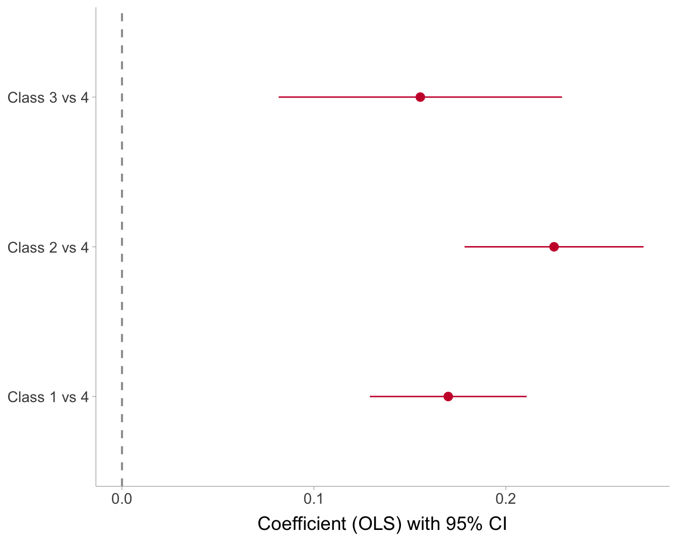
Show the code
coef_df <-
  broom::tidy(m5, conf.int = TRUE) %>%
    mutate(model = "MAP (dummies; ref=Class 4)") %>%
    filter(term != "(Intercept)") %>%
    mutate(
      contrast = case_when(
        term == "class_hat1" ~ "Class 1 vs 4",
        term == "class_hat2" ~ "Class 2 vs 4",
        term == "class_hat3" ~ "Class 3 vs 4",

        term == "sexFemale" ~ "Female (Ref.= Male)",
        term == "educ" ~ "Education (in years)",
        term == "age" ~ "Age",
        term == "income_4Middle-low" ~ "Income Middle-Low",
        term == "income_4Middle-high" ~ "Income Middle-High",
        term == "income_4High" ~ "Income High",
        TRUE ~ term
      ))

coef_df <- coef_df %>%
  mutate(sign = if_else(estimate < 0, "negative", "positive"))

ggplot(coef_df, aes(x = estimate, y = contrast, color = sign)) +
  geom_vline(xintercept = 0, linewidth = 0.7, color = "grey60", linetype = "dashed") +
  geom_pointrange(
    aes(xmin = conf.low, xmax = conf.high),
    fatten = 2,
    size = 1
  ) +
  scale_color_manual(
    values = c("negative" = "black", "positive" = "#ca1137"),
    guide = "none"
  ) +
  labs(x = "Coefficient (OLS) with 95% CI", y = NULL) +
  theme(text = element_text(size = 14))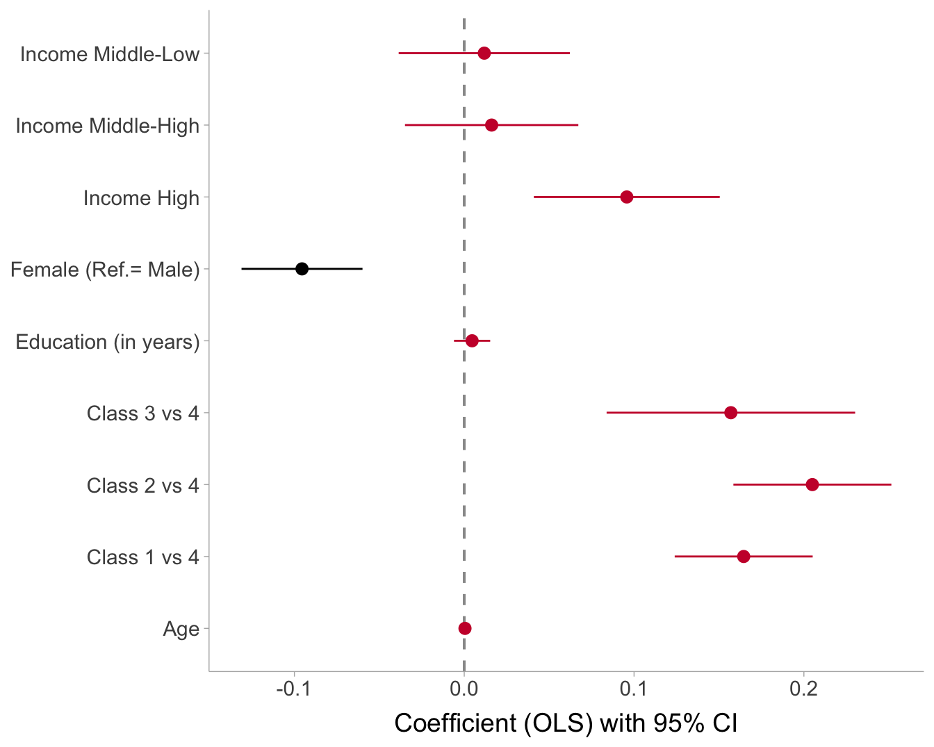
Show the code
coef_df <-
  broom::tidy(m6, conf.int = TRUE) %>%
    slice_tail(n=9) %>%
    mutate(
      contrast = case_when(
        term == "class_hat1:income_4Middle-low" ~ "Class 1 x Income Middle-Low",
        term == "class_hat2:income_4Middle-low" ~ "Class 2 x Income Middle-Low",
        term == "class_hat3:income_4Middle-low" ~ "Class 3 x Income Middle-Low",

        term == "class_hat1:income_4Middle-high" ~ "Class 1 x Income Middle-High",
        term == "class_hat2:income_4Middle-high" ~ "Class 2 x Income Middle-High",
        term == "class_hat3:income_4Middle-high" ~ "Class 3 x Income Middle-High",

        term == "class_hat1:income_4High" ~ "Class 1 x Income High",
        term == "class_hat2:income_4High" ~ "Class 2 x Income High",
        term == "class_hat3:income_4High" ~ "Class 3 x Income High",
        TRUE ~ term
      ))

coef_df <- coef_df %>%
  mutate(sign = if_else(estimate < 0, "negative", "positive"))

ggplot(coef_df, aes(x = estimate, y = contrast, color = sign)) +
  geom_vline(xintercept = 0, linewidth = 0.7, color = "grey60", linetype = "dashed") +
  geom_pointrange(
    aes(xmin = conf.low, xmax = conf.high),
    fatten = 2,
    size = 1
  ) +
  scale_color_manual(
    values = c("negative" = "black", "positive" = "#ca1137"),
    guide = "none"
  ) +
  labs(x = "Coefficient (OLS) with 95% CI", y = NULL) +
  theme(text = element_text(size = 14))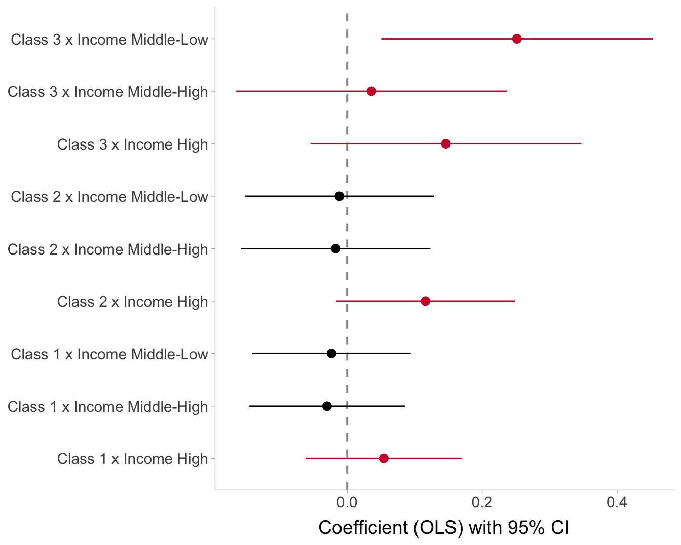
8.2 SEM framework
In this analysis, we will use a structural equation modeling framework to estimate the latent structure of the meritocracy scale and how its dimensions relate to market justice preferences, which are treated as a latent factor of preferences in the areas of pensions, education, and healthcare.
lavaan 0.6-21 ended normally after 49 iterations

  Estimator                                       DWLS
  Optimization method                           NLMINB
  Number of model parameters                        61

  Number of observations                          2521

Model Test User Model:
                                              Standard      Scaled
  Test Statistic                               873.228     790.373
  Degrees of freedom                               124         124
  P-value (Unknown)                                 NA       0.000
  Scaling correction factor                                  1.164
  Shift parameter                                           39.866
    simple second-order correction

Model Test Baseline Model:

  Test statistic                             31744.918   21261.307
  Degrees of freedom                                55          55
  P-value                                           NA       0.000
  Scaling correction factor                                  1.494

User Model versus Baseline Model:

  Comparative Fit Index (CFI)                    0.976       0.969
  Tucker-Lewis Index (TLI)                       0.990       0.986

  Robust Comparative Fit Index (CFI)                            NA
  Robust Tucker-Lewis Index (TLI)                               NA

Root Mean Square Error of Approximation:

  RMSEA                                          0.049       0.046
  90 Percent confidence interval - lower         0.046       0.043
  90 Percent confidence interval - upper         0.052       0.049
  P-value H_0: RMSEA <= 0.050                    0.705       0.979
  P-value H_0: RMSEA >= 0.080                    0.000       0.000

  Robust RMSEA                                                  NA
  90 Percent confidence interval - lower                        NA
  90 Percent confidence interval - upper                        NA
  P-value H_0: Robust RMSEA <= 0.050                            NA
  P-value H_0: Robust RMSEA >= 0.080                            NA

Standardized Root Mean Square Residual:

  SRMR                                           0.039       0.039

Parameter Estimates:

  Parameterization                               Delta
  Standard errors                           Robust.sem
  Information                                 Expected
  Information saturated (h1) model        Unstructured

Latent Variables:
                   Estimate  Std.Err  z-value  P(>|z|)   Std.lv  Std.all
  mjp =~
    just_pension      1.000                               0.716    0.697
    just_educ         1.285    0.037   34.516    0.000    0.920    0.881
    just_healthcar    1.354    0.040   33.647    0.000    0.969    0.924
  perc_merit =~
    perc_effort       1.000                               0.932    0.932
    perc_talent       0.800    0.070   11.457    0.000    0.745    0.745
  perc_nmerit =~
    perc_rch_prnts    1.000                               0.816    0.816
    perc_contact      1.100    0.039   28.390    0.000    0.897    0.897
  pref_merit =~
    pref_effort       1.000                               0.883    0.883
    pref_talent       0.610    0.041   15.024    0.000    0.539    0.539
  pref_nmerit =~
    pref_rch_prnts    1.000                               0.836    0.836
    pref_contact      1.013    0.047   21.561    0.000    0.847    0.847

Regressions:
                   Estimate  Std.Err  z-value  P(>|z|)   Std.lv  Std.all
  mjp ~
    perc_merit        0.047    0.018    2.691    0.007    0.062    0.062
    perc_nmerit      -0.178    0.030   -5.847    0.000   -0.203   -0.203
    pref_merit        0.022    0.029    0.763    0.446    0.027    0.027
    pref_nmerit       0.311    0.021   14.575    0.000    0.363    0.363
    age              -0.002    0.001   -1.741    0.082   -0.002   -0.040
    educ             -0.004    0.010   -0.361    0.718   -0.005   -0.009
    sex_female       -0.211    0.033   -6.423    0.000   -0.295   -0.148
    incom_4Mddl.lw   -0.045    0.045   -1.001    0.317   -0.063   -0.027
    incm_4Mddl.hgh   -0.029    0.046   -0.637    0.524   -0.041   -0.018
    income_4High      0.067    0.051    1.317    0.188    0.094    0.042
    polCenter         0.349    0.066    5.329    0.000    0.488    0.130
    polRight          0.525    0.046   11.500    0.000    0.733    0.327
    polDs.nt.dntfy    0.268    0.041    6.523    0.000    0.374    0.183

Covariances:
                   Estimate  Std.Err  z-value  P(>|z|)   Std.lv  Std.all
  perc_merit ~~
    perc_nmerit      -0.127    0.020   -6.421    0.000   -0.167   -0.167
    pref_merit       -0.036    0.023   -1.583    0.113   -0.044   -0.044
    pref_nmerit       0.157    0.018    8.688    0.000    0.202    0.202
  perc_nmerit ~~
    pref_merit        0.414    0.020   20.931    0.000    0.574    0.574
    pref_nmerit      -0.049    0.017   -2.832    0.005   -0.072   -0.072
  pref_merit ~~
    pref_nmerit       0.040    0.020    2.013    0.044    0.054    0.054

Thresholds:
                   Estimate  Std.Err  z-value  P(>|z|)   Std.lv  Std.all
    just_pensin|t1    0.958    0.144    6.655    0.000    0.958    0.933
    just_educ|t1     -0.361    0.122   -2.964    0.003   -0.361   -0.346
    just_educ|t2      0.740    0.121    6.105    0.000    0.740    0.709
    just_educ|t3      1.567    0.123   12.746    0.000    1.567    1.501
    just_hlthcr|t1   -0.067    0.124   -0.541    0.588   -0.067   -0.064
    just_hlthcr|t2    1.023    0.123    8.294    0.000    1.023    0.976
    just_hlthcr|t3    1.757    0.127   13.819    0.000    1.757    1.675
    perc_effort|t1   -0.881    0.121   -7.310    0.000   -0.881   -0.881
    perc_effort|t2    0.561    0.120    4.685    0.000    0.561    0.561
    perc_effort|t3    1.817    0.126   14.384    0.000    1.817    1.817
    perc_talent|t1   -1.236    0.118  -10.503    0.000   -1.236   -1.236
    perc_talent|t2    0.113    0.116    0.974    0.330    0.113    0.113
    perc_talent|t3    1.543    0.120   12.854    0.000    1.543    1.543
    prc_rch_prnt|1   -2.500    0.116  -21.461    0.000   -2.500   -2.500
    prc_rch_prnt|2   -1.837    0.119  -15.374    0.000   -1.837   -1.837
    prc_rch_prnt|3   -0.792    0.118   -6.708    0.000   -0.792   -0.792
    perc_contct|t1   -2.350    0.123  -19.113    0.000   -2.350   -2.350
    perc_contct|t2   -1.950    0.121  -16.062    0.000   -1.950   -1.950
    perc_contct|t3   -0.584    0.121   -4.841    0.000   -0.584   -0.584
    pref_effort|t1   -1.661    0.130  -12.777    0.000   -1.661   -1.661
    pref_effort|t2   -1.111    0.126   -8.827    0.000   -1.111   -1.111
    pref_effort|t3    0.152    0.126    1.209    0.227    0.152    0.152
    pref_talent|t1   -1.217    0.117  -10.365    0.000   -1.217   -1.217
    pref_talent|t2   -0.016    0.114   -0.139    0.889   -0.016   -0.016
    pref_talent|t3    1.166    0.116   10.086    0.000    1.166    1.166
    prf_rch_prnt|1   -1.225    0.115  -10.617    0.000   -1.225   -1.225
    prf_rch_prnt|2   -0.180    0.115   -1.563    0.118   -0.180   -0.180
    prf_rch_prnt|3    1.308    0.117   11.183    0.000    1.308    1.308
    pref_contct|t1   -0.911    0.114   -7.958    0.000   -0.911   -0.911
    pref_contct|t2    0.254    0.115    2.207    0.027    0.254    0.254
    pref_contct|t3    1.594    0.118   13.488    0.000    1.594    1.594

Variances:
                   Estimate  Std.Err  z-value  P(>|z|)   Std.lv  Std.all
   .just_pension      0.542                               0.542    0.514
   .just_educ         0.244                               0.244    0.224
   .just_healthcar    0.161                               0.161    0.147
   .perc_effort       0.131                               0.131    0.131
   .perc_talent       0.444                               0.444    0.444
   .perc_rch_prnts    0.334                               0.334    0.334
   .perc_contact      0.195                               0.195    0.195
   .pref_effort       0.220                               0.220    0.220
   .pref_talent       0.709                               0.709    0.709
   .pref_rch_prnts    0.302                               0.302    0.302
   .pref_contact      0.283                               0.283    0.283
   .mjp               0.358    0.021   17.341    0.000    0.698    0.698
    perc_merit        0.869    0.075   11.605    0.000    1.000    1.000
    perc_nmerit       0.666    0.026   25.193    0.000    1.000    1.000
    pref_merit        0.780    0.053   14.680    0.000    1.000    1.000
    pref_nmerit       0.698    0.033   20.947    0.000    1.000    1.000

R-Square:
                   Estimate
    just_pension      0.486
    just_educ         0.776
    just_healthcar    0.853
    perc_effort       0.869
    perc_talent       0.556
    perc_rch_prnts    0.666
    perc_contact      0.805
    pref_effort       0.780
    pref_talent       0.291
    pref_rch_prnts    0.698
    pref_contact      0.717
    mjp               0.302
References
Castillo, J. C., Iturra, J., Maldonado, L., Atria, J., & Meneses, F. (2023). A Multidimensional Approach for Measuring Meritocratic Beliefs: Advantages, Limitations and Alternatives to the ISSP Social Inequality Survey. International Journal of Sociology, 53(6), 448–472. https://doi.org/10.1080/00207659.2023.2274712